
In the previous post, we performed thermal analysis for conduction. In this post, we are going to perform thermal analysis using conduction as well as convection. If you have not read the post on thermal analysis using conduction you can check it out here.
Performing Heat Transfer Analysis
For this tutorial, we will be using a pipe, applying a flux load to one face, and attaching an ambient temperature constraint near another face to analyze the behavior of the component.
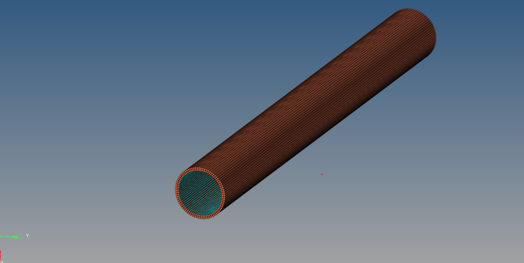
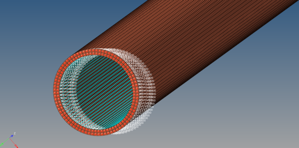
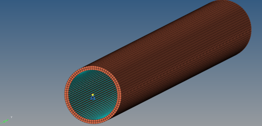
Meshed Model
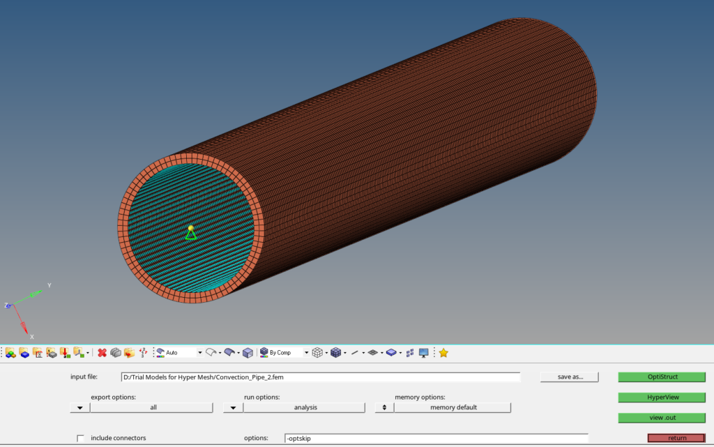
In this tutorial, we will be using a pipe with ID 36 and OD 42 meshed using Hex elements of size 2 as shown in the image below.
Defining Thermal Elements
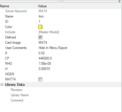
To perform the thermal analysis we need to define the material for thermal elements. Material for thermal elements can be defined using the MAT4 card image and requires heat transfer coefficient and density inputs. You can read more about materials and property here. To define a new material we can right-click on the white browser-area and then go to Create -> Material. We will name this material as Iron. We will put the values for the material as shown in the image below.

Next, we have to create a property for this we can again right-click on the white browser area and then go to Create -> Property. We will name this property as Solid_Property.
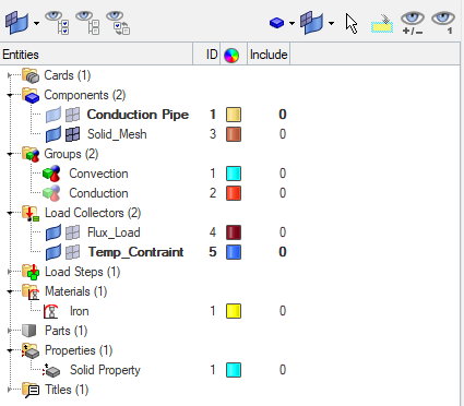
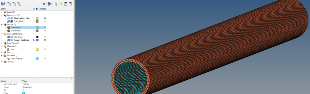
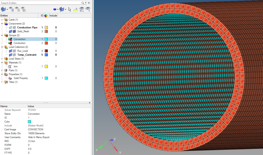
Now we have to create groups to define which elements will be used for thermal analysis. To do this we can right-click on the white browser area and then go to Create -> Groups. We will name this group as Conduction and then select the elements under this group. We will select elements on one end face of the pipe. Next, we will create a new group in the same way and name it Convection, and then select the elements on the inner face of the pipe.
Boundary Conditions
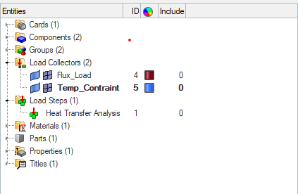
To apply boundary conditions we have to first create load collectors for the same. We can right-click on the white browser area and then go to Create -> Load Collector. We will name this load collector as flux load. Then to create the thermal load we can go to Analysis -> Flux, and then select the elements on which the flux load will be applied, i.e. the elements under the conduction group as shown in the image below. We will keep the flux value at 0.6.
Now we will create a temporary node in the vicinity of the end face of the pipe opposite the face where the flux load is applied.
Then we will create a new load collector by again right-clicking on the white browser area and then going to Create -> Load Collector. We will name this load collector temp_constraint. Then we will create temperature constraints by going to Analysis -> Constraints. Then uncheck all the dofs and then go to create/edit and put D as 18, this is the temperature constraint. We will select the temporary node created for applying temperature constraints as shown in the image below.
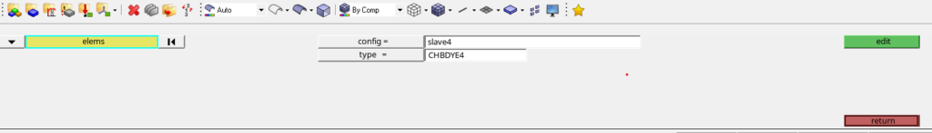
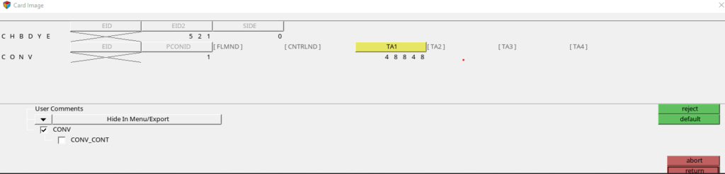
Creating the constraint on the node will not be enough as it is not linked to the pipe. We have to link the node with the temperature constraint to the convection group for the convection to take place. We can do this by going to card edit and selecting the convection element by group and then selecting config as SLAVE4 and type as CHBDYE, then clicking on create/edit, and then selecting the temperature constraint node under TA field.
Analysis Setup
Next, we will create a Load Step by right-clicking on the white browser area and then going to Create -> Load Step, we will name this load step as Thermal analysis. We will change the analysis type from generic type to Heat Transfer (Static), and then we will reference temp_constraint under the SPC field and Flux_load under the load field.
Performing Analysis
To perform the analysis, we will go to Analysis -> Optistruct as shown in the below image, and then click on Optistruct to run the analysis. Kindly note that we are using Optistruct for this tutorial and you can use any other solver of your choice too and the output cards have to be defined accordingly.
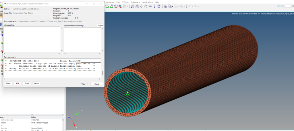
Once you click the Optistruct a pop-up will occur as shown in the image below showing the progress of the run for the solver.
Output
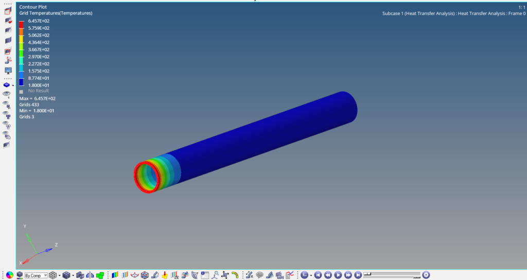
Once the solver run is completed we can view the output values we can also go to View -> Output file. To visualize the results we can go to Results, which will open Hyperview. We can analyze the temperature gradients under the thermal load conditions as shown in the image below.
So to summarise what have we done in this tutorial.
- Create a meshed model of the buckling column.
- Apply the material and property to the model.
- Apply boundary conditions.
- Create two load steps one for linear static analysis and the other for linear buckling analysis.
- Run the model in the solver to view the results.
For better visualization, you can also refer to the below video.
This is all for this post see you all in the next post. Don’t forget to follow my Facebook and Instagram Page. Till then keep learning.