
In this post, we will learn and perform Thermal analysis in Hypermesh.
We will start with understanding Thermal load, and what constitutes the thermal loads, and then finally prepare a model and perform Thermal analysis.
What are Thermal loads?
Thermal loads are created when there is heat transfer due to the temperature difference between the subject and the environment. Heat transfer is the transfer of energy from one place to another, i.e. it occurs when thermal energy moves from one place to another.
Types of Heat transfer
Heat can be transferred through the below-mentioned ways.
- Conduction: This type of heat transfer occurs when heat is transferred between solids in contact. So solids are the medium of transfer here.
- Convection: This type of heat transfer occurs when heat is transferred between solid and gas or solid and liquid in contact. So basically fluids are the medium of transfer here.
- Radiation: This type of heat transfer occurs when heat is transferred without a medium, i.e. through electromagnetic waves.
Performing Heat Transfer Analysis
For this tutorial, we will be using a pipe and applying a flux load to it.
Meshed Model
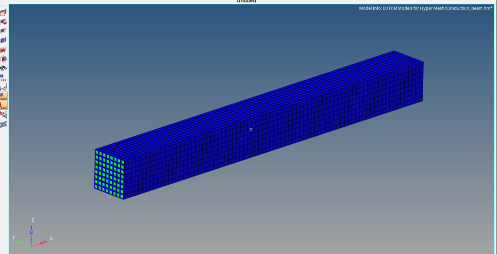
In this tutorial, we will be using a beam of dimension 8 mm x 8 mm x 80 mm meshed using Hex elements of size 1 as shown in the image below.
Defining thermal elements
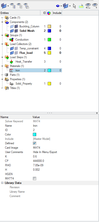
To perform the thermal analysis we need to define the material for thermal elements. Material for thermal elements can be defined using the MAT4 card image and requires heat transfer coefficient and density inputs. You can read more on material and properties in hypermesh here. To define a new material we can right-click on the white browser-area and then go to Create -> Material. We will name this material as Iron. We will put the values for the material as shown in the image below.
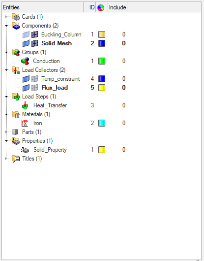
Next, we have to create a property for this we can again right-click on the white browser area and then go to Create -> Property. We will name this property as Solid_Property. Now we have to create groups to define which elements will be used for thermal analysis. To do this we can right-click on the white browser area and then go to Create -> Groups. We will name this group as Conduction and then select the elements under this group. We will select elements on one 8 mm x 8mm face of the beam under this group.
Boundary Condition
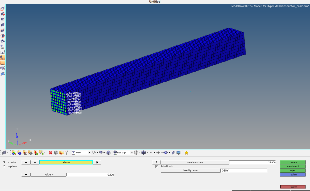
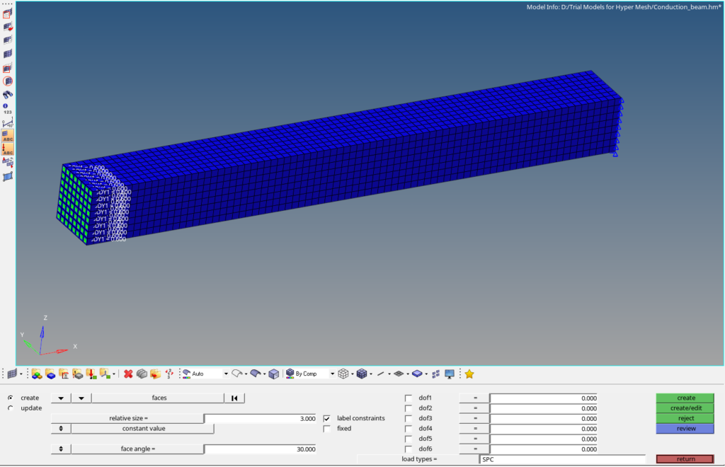
To apply boundary conditions we have to first create load collectors for the same. We can right-click on the white browser area and then go to Create -> Load Collector. We will name this load collector as flux load. Then to create the thermal load we can go to Analysis -> Flux, and then select the elements on which the flux load will be applied, i.e. the elements under the conduction group as shown in the image below. We will keep the flux value at 0.6.
Then we will create a new load collector by again right-clicking on the white browser area and then going to Create -> Load Collector. We will name this load collector temp_constraint. Then we will create temperature constraints by going to Analysis -> Constraints. Then uncheck all the dofs and then go to create/edit and put D as 18, this is the temperature constraint. We will select the face opposite to the face on which flux load is applied.
Analysis Setup
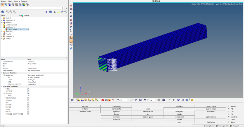
Next, we will create a Load Step by right-clicking on the white browser area and then going to Create -> Load step, we will name this load step as thermal analysis. We will change the analysis type from generic to Heat transfer (static), and then we will reference the temp_constraint load collector under the SPC field and flux under the Load field.
Performing Analysis
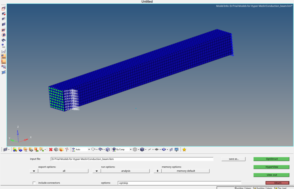
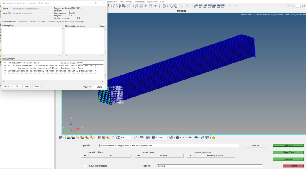
To perform the analysis, we will go to Analysis -> Optistruct as shown in the below image, and then click on Optistruct to run the analysis. Kindly note that we are using Optistruct for this tutorial and you can use any other solver of your choice too and the output cards have to be defined accordingly.
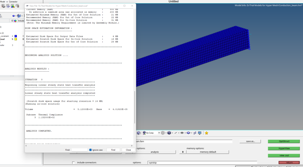
Once you click the Optistruct a pop-up will occur as shown in the image below showing the progress of the run for the solver.
Output
Once the solver run is completed we can view the output values we can also go to View -> Output file as shown in the image below.
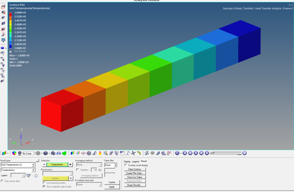
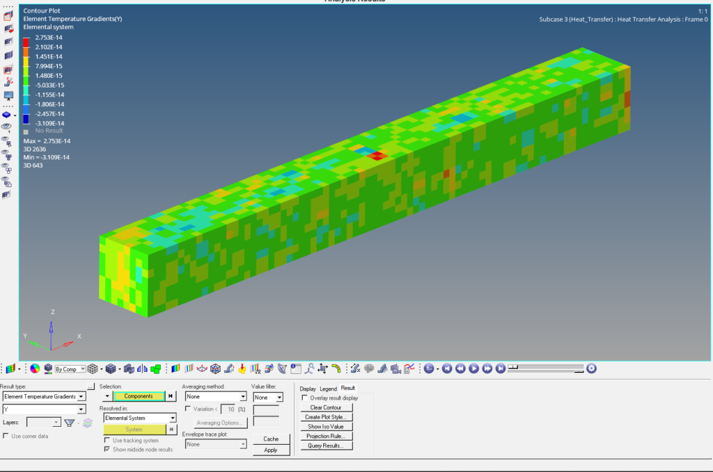
To visualize the results we can go to Results, which will open Hyperview. We can analyze the temperature gradients under the thermal load conditions as shown in the image below.
So to summarise what have we done in this tutorial.
- Create a meshed model of the buckling column.
- Apply the material and property to the model.
- Apply boundary conditions.
- Create two load steps one for linear static analysis and the other for linear buckling analysis.
- Run the model in the solver to view the results.
For better visualization, you can also refer to the below video.
This is all for this post see you all in the next post. Don’t forget to follow my Facebook and Instagram Page. Till then keep learning.