Till now, we have seen static Frequency response analysis before. If you have not seen that post, you can check it out here. In this post, we are going to discuss something similar, known as Random Vibration.
We will start by understanding what Random Vibration Analysis is, and then we will proceed to perform the analysis.
What is Random Vibration?
Random vibration refers to motion caused by non-periodic, unpredictable forces. Unlike harmonic vibrations (e.g., sine waves), these forces vary in amplitude and frequency without a fixed pattern. Examples of sources are wind gusts on buildings, road roughness affecting vehicles, turbulence in aerospace structures, and earthquake ground motion.
Random vibration analysis is a statistical method used to predict how a system or structure will behave under random, unpredictable, non-repeating forces like wind, earthquakes, or road noise. Instead of analyzing one specific force, it uses probability distribution, power spectral density (PSD), and response spectra to model the range of possible excitations.
It is commonly applied in structural engineering, automotive, aerospace, and electronics to ensure durability and reliability.
Performing Random Vibration Analysis
For this tutorial, we will use a plate, subject it to a certain frequency range, and analyze its behavior.
Meshed Model
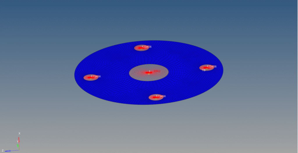
In this tutorial, we will be using a plate with 5 holes and mesh with 2D elements, fix the plate with the 4 holes on the periphery, and apply a load on the central hole as shown in the image below:

Boundary Conditions
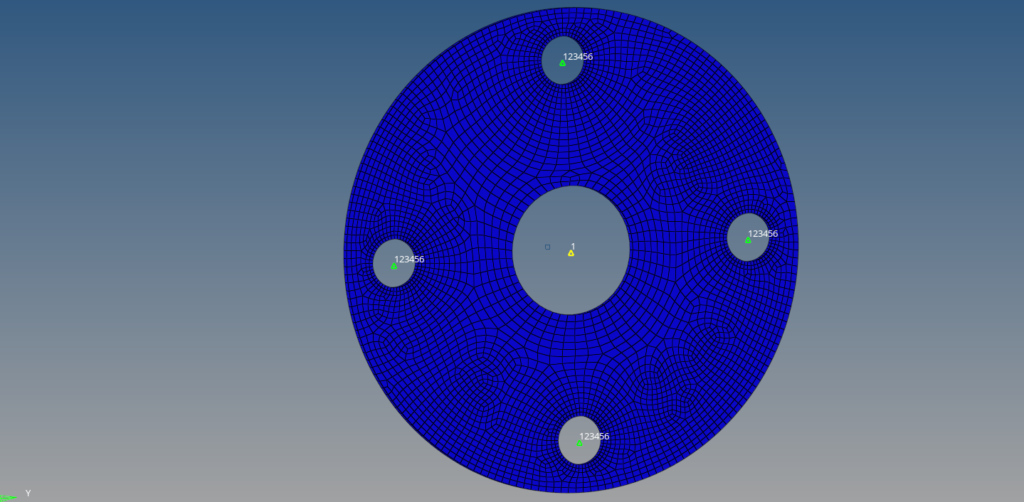
To apply the boundary conditions, first, we need to create RBE2 elements connecting the nodes on the periphery of the holes to a master node, as shown in the image below.
Next, we will constrain the four holes on the periphery of the circular plate. For this, we will create a load collector by right-clicking on the white browser area and going to Create -> Load Collectors. We will name this load collector as constraints. We can create the constraints by going to Analysis -> Constraints and selecting the master nodes of the RBE2 elements for those holes.
Now we have to create a DAREA load collector. We can again right-click on the white browser area and go to Create -> Load Collectors. We will name this load collector DAREA. We can create this load collector by going to Analysis -> Constraints and selecting only the dof that is perpendicular to the plate, that is dof2 (y-axis). In this case, we will change the card image of this load collector to DAREA. Select the master node of the central hole to apply this load collector.
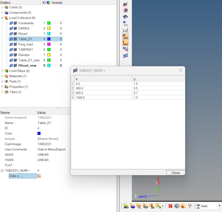
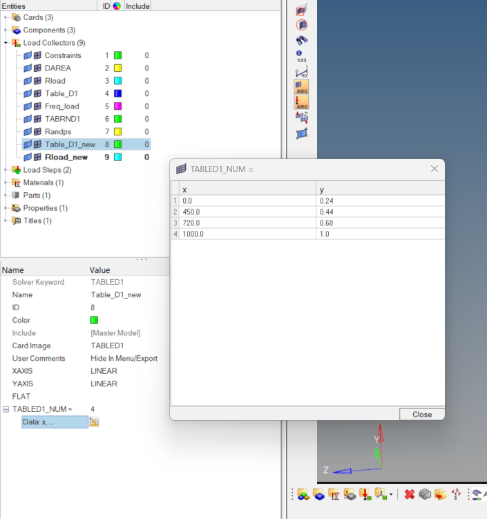
Next, we have to create two TABLED1 load collectors. This load collector is created to define the frequency range and the frequency function. We can create the load collector by right-clicking on the white browser area and then going to Create -> Load Collectors. We will name these load collectors Table_D1 and Table_D1_new. Now change the card image of these load collectors to TABLED1. Then add the data in the two load collectors as shown in the image below.
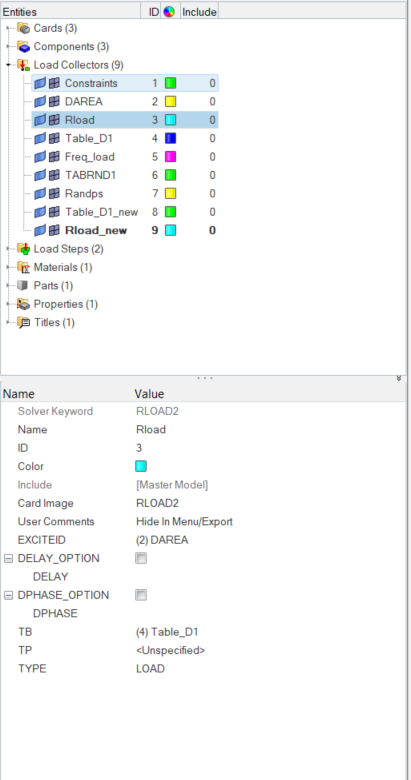
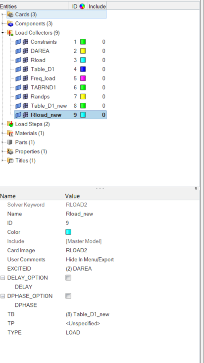
Now we will create RLOAD load collectors. This load collector is used to couple the DAREA and TABLED1 load collectors. We can right-click on the white browser area and then go to Create -> Load Collectors. We will name these load collectors as Rload and Rload_new. Change the card image of the load collector to RLOAD2. Select the respective TABLED1 load collector under the TB field and the DAREA load collector under the EXCITEID field.
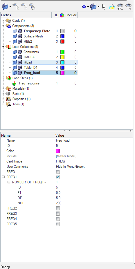
Next, we will have to create a Frequency load collector. This load collector will have the Frequency load. For this, we can again right-click on the browser area and go to Create -> Load Collectors. We will name this load collector as Freq_load. Next, we have to give the starting frequency as 0 under the F1 field, an incremental frequency of 5 under the DF field, and the number of data points as 200 under the NDF field, as shown in the image below.
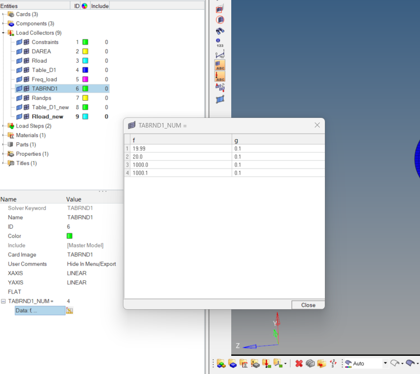
Next, we will have to create a TABRND1 load collector. This load collector will have a Random Frequency. For this, we can again right-click on the browser area and go to Create -> Load Collectors. We will name this load collector as TABRND1. Next, we will fill in the data in the table, as shown in the image below.
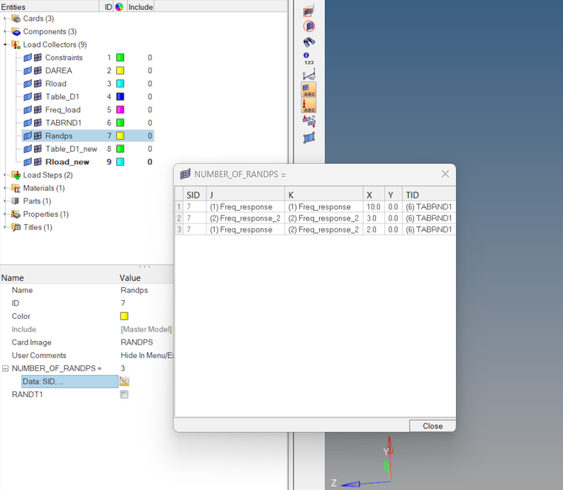
Next, we will have to create a RANDPS load collector. This load collector will couple the load steps. For this, we can again right-click on the browser area and go to Create -> Load Collectors. We will name this load collector as Randps. Next, we will fill in the data in the table, as shown in the image below.
Analysis Setup
We have to apply material, property, now, and create a load step.
Create a PSHELL property by right-clicking on the white area in the browser area and selecting Create -> Property, then select the card image as PSHELL and assign this property to the plate component. Enter the shell thickness as 2.
Then, create a material by right-clicking on the white browser area and going to Create -> Material. We will use steel for this tutorial; the values of steel are available by default in Hypermesh.
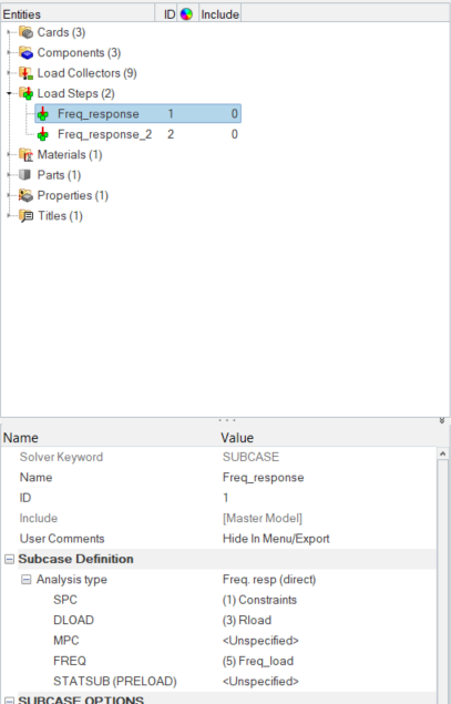
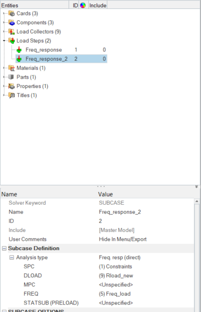
Then, create two Load steps by right-clicking on the white browser area and going to Create -> Load Step. Name these load steps as Freq_response and Freq_response_2, and then select the Analysis type as Frequency Response Direct. Select the constraints load collector under the SPC field and the Frequency load collector under the FREQ field, and the respective Rload under the DLOAD field. Once completed, the browser area will look very similar to the image below.
Performing Analysis
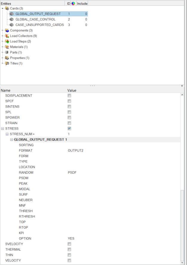
First, we will select the output cards required for the analysis. We can do this by going to Analysis -> Control Cards -> Global Output Requests. We will select the Stress output cards. Under this card, we will select the output format as OUTPUT2 and Random as PSDF.
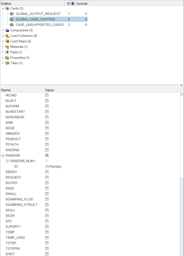
Next, we will select the Global case control cards in the same way and select the Random card under it, and select the Randps load collector under the ID.
Next, we will select the case_unsupported_cards and insert the card name as shown in the image below.

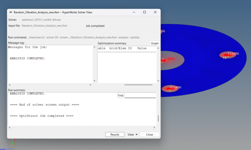
To perform the analysis, we will go to Analysis -> Optistruct, and a window similar to the one below will appear. Kindly note that we are using Optistruct for this tutorial.
If the Optistruct option is not appearing under Analysis in the toolbar. Then go to Preference -> User Profile and select Optistruct. Select export options as custom, run options as Analysis, and keep the memory option as default. Then click on Optistruct to run the analysis. A pop-up window will appear displaying the progress of the run as shown in the image below.
Output
Once the solver run is completed, we can view the output values. We can also go to View -> Output file as shown in the image below.
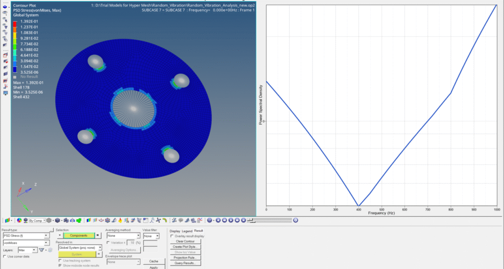
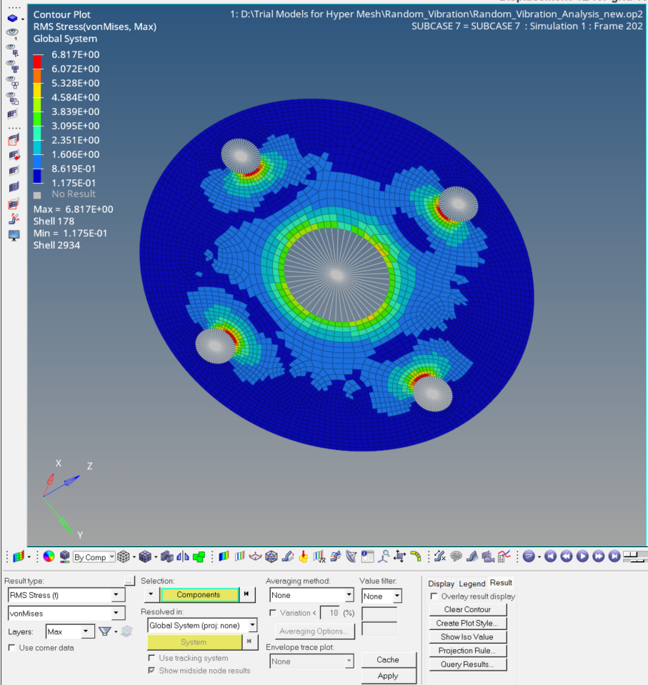
Click on Results to view the results of the Analysis as shown in the image below. A window like the image below will open. This is the Hyperview window and is used to see the results of the analysis.
You can also refer to the video below for more clarity on the topic.
This is all for this post. See you all in the next post. Don’t forget to follow my Facebook and Instagram Pages. Till then, keep learning.
This is all for this post. Hope you got to learn something new from this post. Don’t forget to follow my Facebook and Instagram pages for regular updates. See you all in the next post. Till then, keep learning.