
In this post, we are going to learn and perform Linear Buckling analysis in Hypermesh.
So we will be starting with knowing what is buckling analysis, preparing a model to use, applying boundary conditions and then performing modal analysis, and finally comparing the results. Before diving into the tutorial we need to get familiar with some terms.
What is Buckling?
Buckling by definition is sudden deformation in the component or structure under compression when the compression load reaches a certain critical value. This critical buckling load is calculated using Euler’s buckling formula which uses Young’s modulus, second moment of area, and the effective length of the component. You can read more about buckling here.
Performing Buckling Analysis
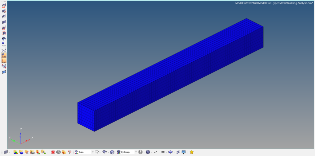
For this tutorial, we will be using a rectangular column under compression load to perform buckling analysis.
Meshed Column Model
For this tutorial, I have used an 8 mm x 8 mm x 80 mm column. I have used the Hexa element to mesh the column.
Boundary Condition
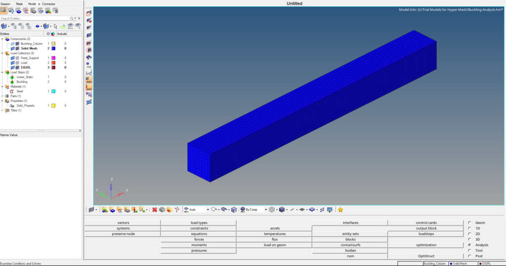
To apply boundary conditions we need to create load collectors. We will first create a load collector named Fixed_support and fix all the degrees of the bottom face of the column. To create this we can go to Analysis -> Constraints. Now we will create a load collector named Load and apply the load on the top face of the column. We will keep the load value as 5600 KN.
Then we need to create a load collector EIGRL having card image as EIGRL. This load collector is used to extract the modes of buckling for the column. To create a new load collector we can right-click on the white browser area, then go to Create -> Load Collector. If you want to understand more about modes you can read this post here on Modal Analysis.
Analysis Setup
We now have to apply material, and property, and create load steps.
We will create a property load collector named Solid Property with card image PSOLID. We can create the property by right-clicking on the white browser area and then going to Create -> Property. Then create a material load collector named Steel by again going to the white browser area right-clicking on it and going to Create -> Material. We will be using steel for this tutorial, it is the material whose values are available by default in Hypermesh.
Next, we have to create a load step named Linear Static for Linear Static Analysis. We can do this by right-clicking on the white browser area and then going to Create -> Load Step. Select the analysis type as Linear Static and reference the Fixed_support and Load load collectors in the SPC and load fields in this load step. After this, we need to create another load step named buckling for buckling analysis. Create a new load step by following the steps followed before and then select the analysis type as buckling and reference the EIGRL load collector in the method(struct) field and the constraint load collector in the SPC field.

Performing Analysis
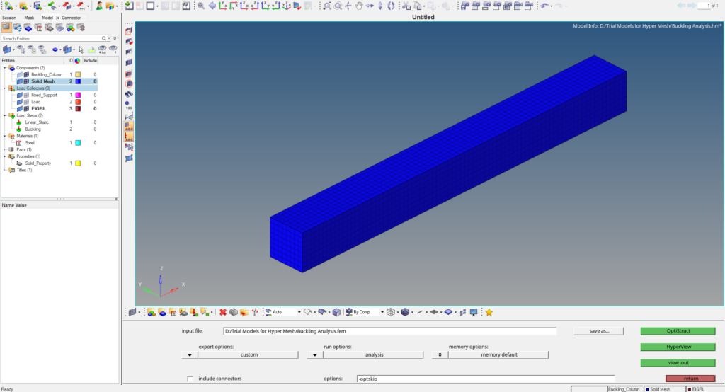
To perform the analysis, we will go to Analysis -> Optistruct as shown in the below image, and then click on Optistruct to run the analysis. Kindly note that we are using Optistruct for this tutorial and you can use any other solver of your choice too.
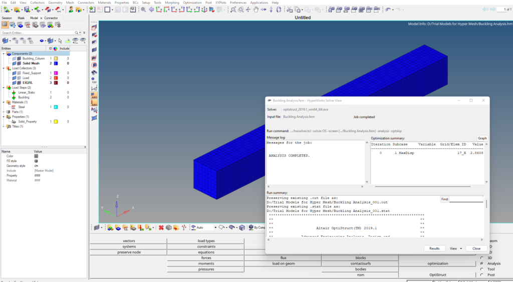
Once you click the Optistruct a pop-up will occur as shown in the image below showing the progress of the run for the solver.
Output
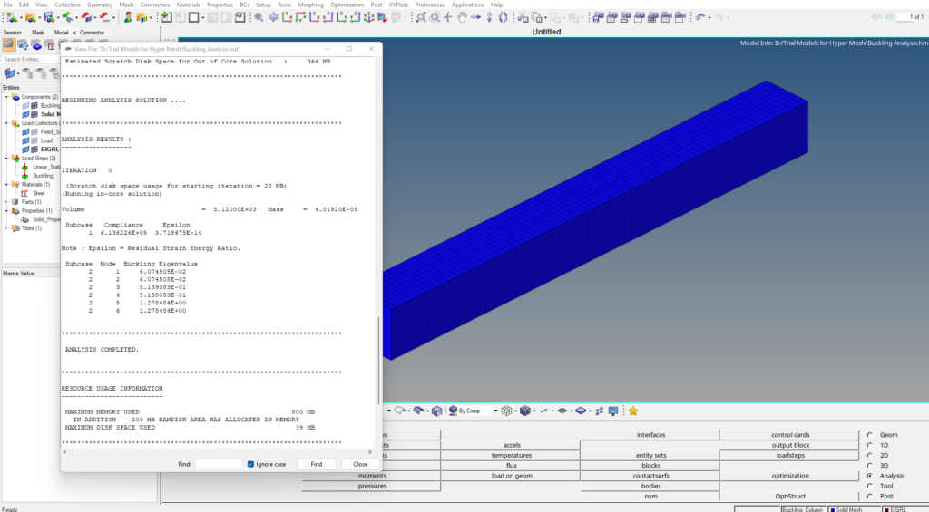
Once the solver run is completed we can view the output values we can also go to View -> Output file as shown in the image below.
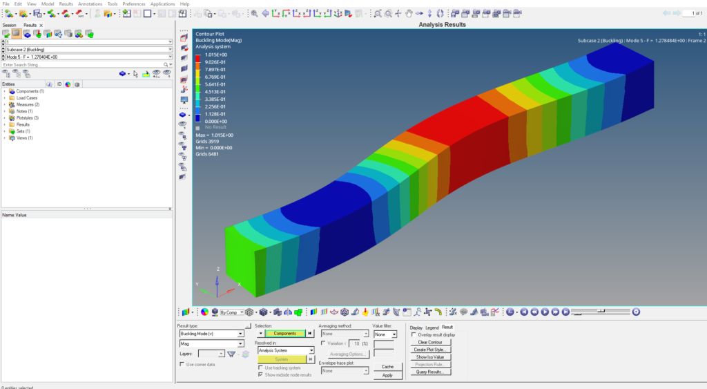
To visualize the results we can go to Results, which will open Hyperview. We can analyze the deformation of the structure under different load conditions as shown in the image below.
So to summarise what we have done in this tutorial:
- Create a meshed model of the buckling column.
- Apply the material and property to the model.
- Apply boundary conditions.
- Create two load steps one for linear static analysis and the other for linear buckling analysis.
- Run the model in the solver to view the results.
You can also refer to the below video for more clarity on this tutorial.
This is all for this post see you all in the next post. Don’t forget to follow my Facebook and Instagram Page. Till then keep learning.