In the previous posts, we have seen analyses where a body is constrained and subjected to loading. If you have not seen those posts you can check them out here. In this post, we will see something different from the usual analyses. In this post, we are going to perform Inertia Relief Analysis.
So let’s start by understanding what inertia Relief is and then we will proceed to perform the analysis.
What is Inertia Relief Analysis?
Inertia Relief as the name suggests is used to relieve the free or partially constrained structure of the applied forces by applying inertial forces.
This technique is particularly useful for analyzing structures that are not fully constrained, such as aircraft in flight or satellites in space, where traditional boundary conditions cannot be applied.
Performing Inertia Relief Analysis
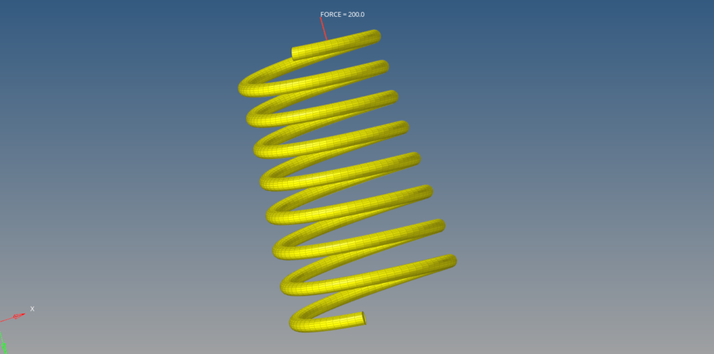
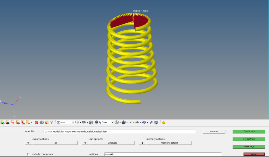
For this tutorial, we will use a toy spring and apply force on a section of the top part of the spring.
Meshed Model
I have meshed the spring with Hex elements as shown in the image below:
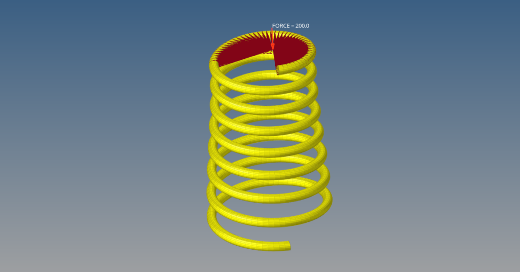
Boundary Conditions
For this analysis, we will apply a load of 200 N in the Y direction. We can do this by going to Analysis -> Forces, selecting the master node of the created RBE2 element, and selecting the direction as Y. Refer to the image below.
Analysis Setup
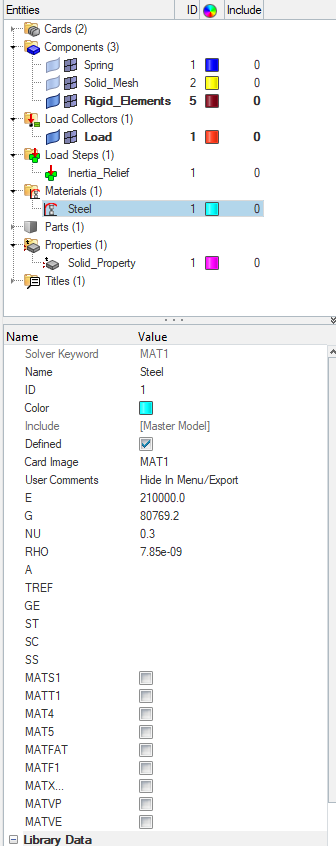
We have to create the spring material. We can do this by right-clicking on the white browser area and then going to Create -> Material. We will use the default material, Steel, as shown in the image below.
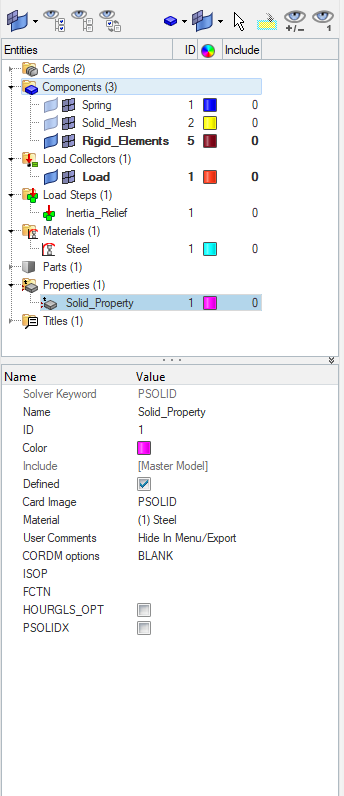
Next, we need to create a property for the component. We can do this by right-clicking on the white browser area and then going to Create -> Property. We will select the card image for this property as PSOLID as this will be for a solid component. Refer to the image below.
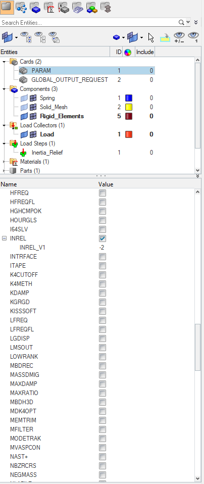
Next, we need to create some control cards for the analysis. We can do this by going to Analysis -> Control Cards -> PARAM -> INREL and selecting INREL_V1 as -2 as shown in the image below.
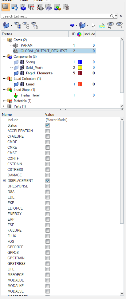
We will also select outputs by going to Analysis -> Control Cards -> Global_Output_Request and selecting Displacement, Stress and Strain and output format as H3D.
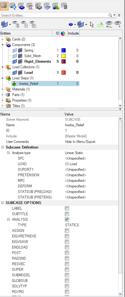
Next, we will create a Load Step by right-clicking on the white browser area and then going to Create -> Load Step, we will name this load step as Inertia_Relief. We will change the analysis type from generic type to Linear Static, and then we will reference Load under the load field.
Performing Analysis
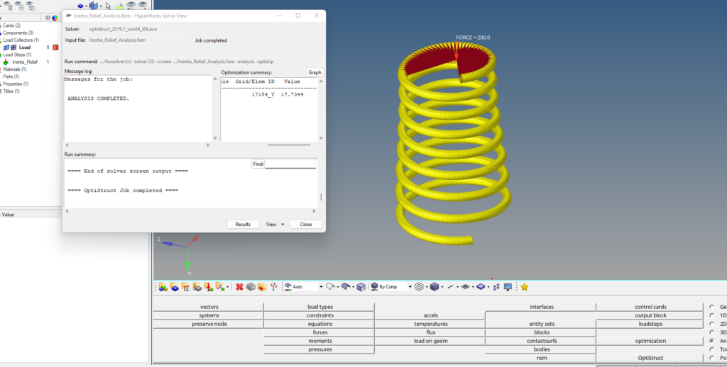
To perform the analysis, we will go to Analysis -> Optistruct as shown in the below image, and then click on Optistruct to run the analysis. Kindly note that we are using Optistruct for this tutorial and you can use any other solver of your choice too; the output cards have to be defined accordingly.
Once you click the Optistruct a pop-up will occur as shown in the image below showing the progress of the run for the solver.
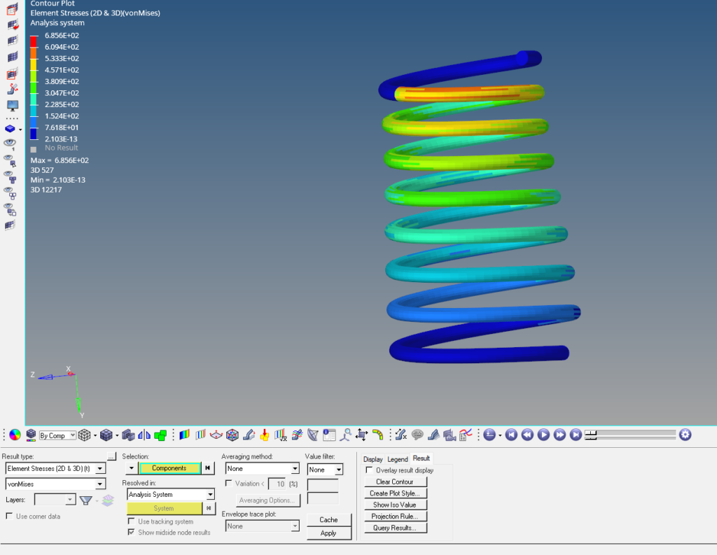
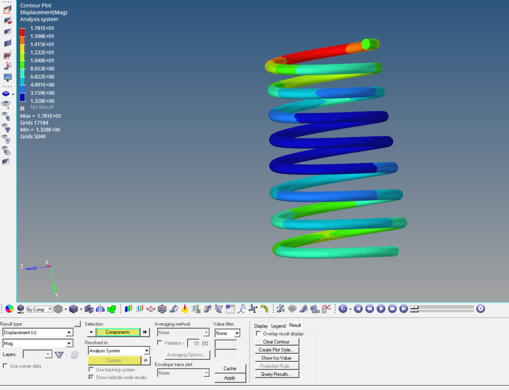
Output
Once the solver run is completed we can view the output values we can also go to View -> Output file. To visualize the results we can go to Results, which will open Hyperview. We can analyze the temperature gradients under the thermal load conditions as shown in the image below.
You can also refer to the video below for more clarity on the topic.
This is all for this post see you all in the next post. Don’t forget to follow my Facebook and Instagram Pages. Till then keep learning.