
In the previous post, we performed a Crash analysis. If you have not seen that post you can find it here. In this post, we will conduct an Impact Analysis using Hypermesh and Radioss.
So first of all let’s start by understanding impact analysis and its use cases.
What is Impact Analysis?
Impact Analysis as the word states is used to study the effect on the body when it comes under sudden impact from a body more rigid than it. The thing we will observe here is how energy is dissipated and how the stress is developed. If you would have studied elementary physics you would know that there are two types of collisions, namely elastic and inelastic collision, and there is an exchange or transfer of energy during collision.
This analysis is relevant in the arms, automotive, and other industries where the object can be subject to sudden impact. In Crash Analysis we had crashed the body or subject with a rigid object, here the body or subject is stationary and comes in contact with a moving rigid body.
Performing Impact Analysis
For this tutorial, we will use a 9 mm bullet traveling at a speed of 5 m/s and colliding with a surface such as a wall or bullet-proof glass. We will observe its effect on the surface.
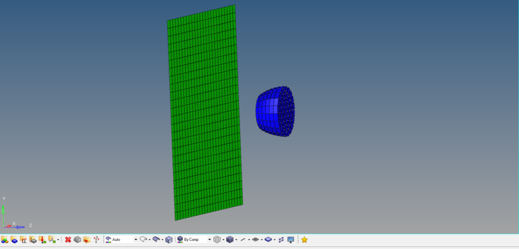
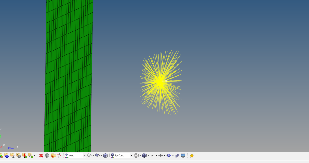
Meshed Model
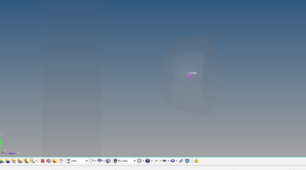
In this tutorial, we will be using a 9 mm bullet and a surface meshed with 2D elements of mixed type, the bullet is traveling at a speed of 5 m/s. I have also created a Rigid Element as shown in the images below:
Boundary Conditions
Post meshing the bullet we need to give the boundary conditions.
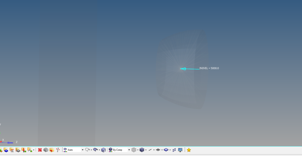
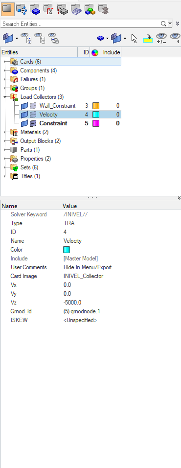
Here we will give the bullet an initial velocity of 5 m/s. For this, we can go to Tools -> BCs Manager to create the initial velocity Load Collector with card image as INVEL_Collector and select the rigid element component collector created to assign velocity. Here I have used the velocity as -5000 in the z field as the bullet is pointing towards negative Z-direction and the unit of velocity is mm/s in Hypermesh as shown in the below image.
Next, we need to constrain the translational along other axes apart from Z and the rotational motion of the bullet along all the axes. For this again we can to Tools -> BCs Manager and create a load collector named constraint with card image as BCs_Collector, and apply the constraint to the rigid element component collector.
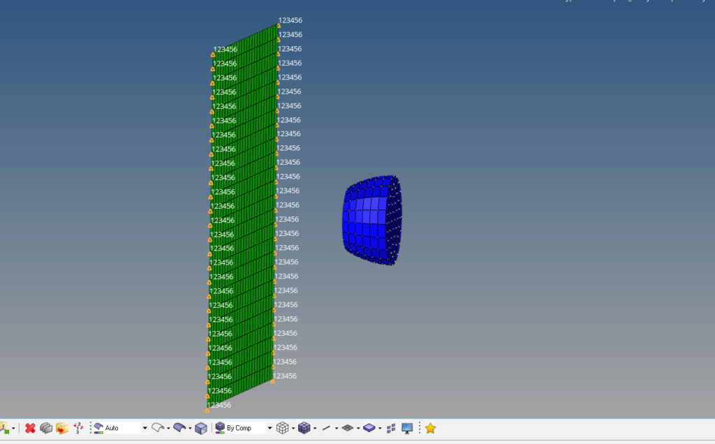
Next, we will constrain the edges of the surface to observe the impact of the bullet on it. We will constrain all the degrees of freedom of the nodes on the edge of the wall. For this, we can again go to Tools -> BCs Manager and create a load collector named Wall_Constraint with a card image as BCs_Collector, and apply the constraint to the rigid element component collector.
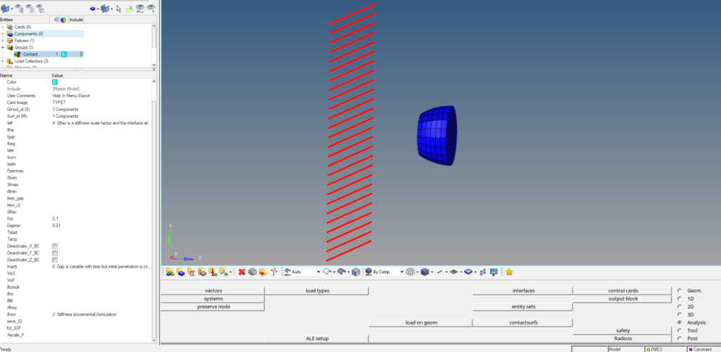
Next, we will need to define the contacts for the bullet. For this, we can right-click on the white browser area and then go to Create -> Contact. Here we will select the card image of contact as TYPE 7, select the wall component as the slave and the bullet component as the master entity, and Istf (stiffness definition) as “4. Stfac is a stiffness scale factor and the interface stiffness is computed from both master and slave characteristics”, Fric as 0.1, Gapmin as 0.01, and Inacti as “6 Gap is variable with time but initial penetration is computed”, Iform as “2. Stiffness (incremental) formulation”.
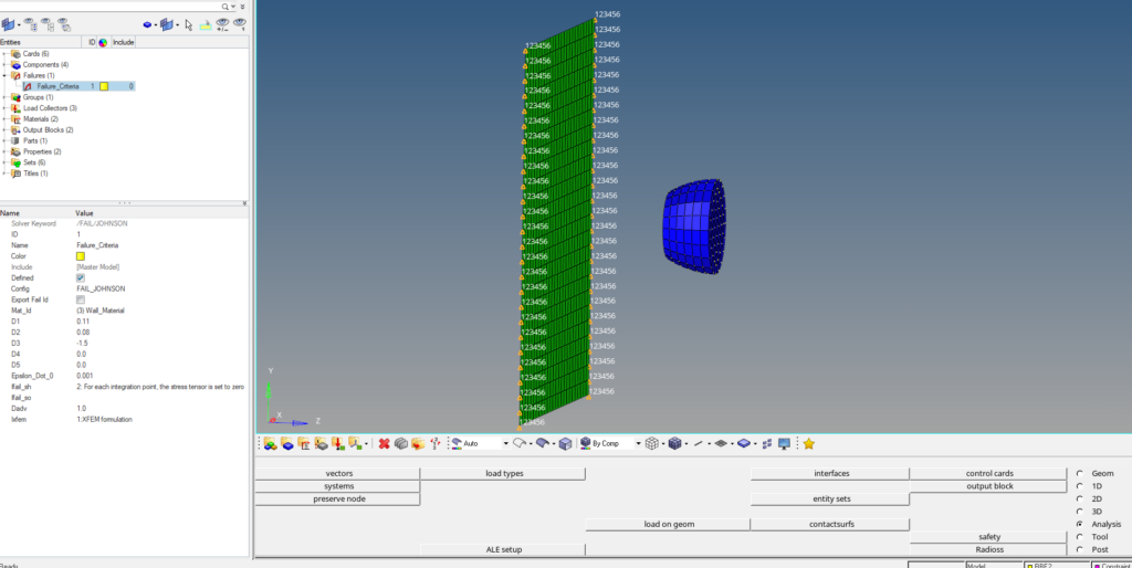
Next, we have to set up failure criteria for the surface. For this, we can again right-click on the white browser area and then go to Create ->Failure. Here we have to select the wall_material under the Mat_Id. Refer to the image below for more clarity.
Analysis Setup
We now have to apply the material and property.
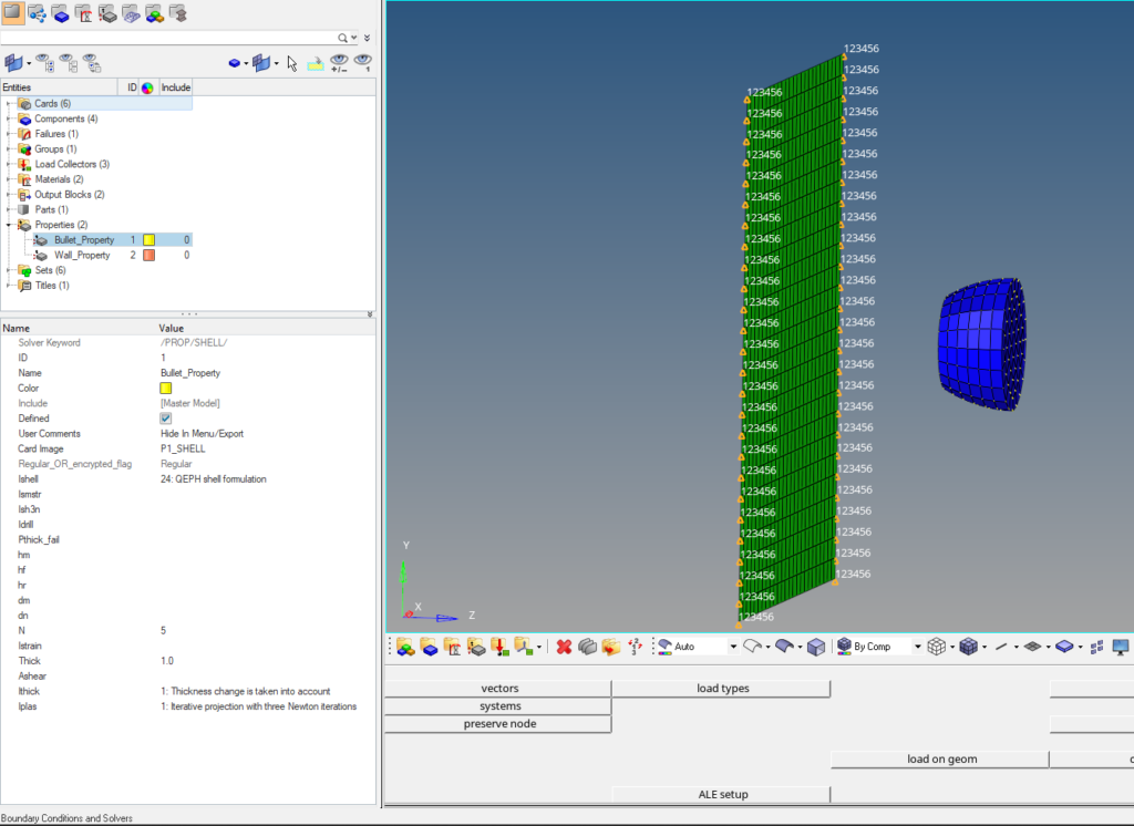
Create a PSHELL property by right-clicking on the white area on the browser area and selecting Create -> Property, we will name this property Bullet_Property, then select the card image as P1_SHELL, and put Ishell as “24 QEPH shell formulation”, N as 5, Thick as 1, Ithick as “1 Thickness change is taken into account”, Iplas as “1 Iterative projection with three Newton Iterations”, and assign this property to the bullet component. Refer to the image below for more clarity.
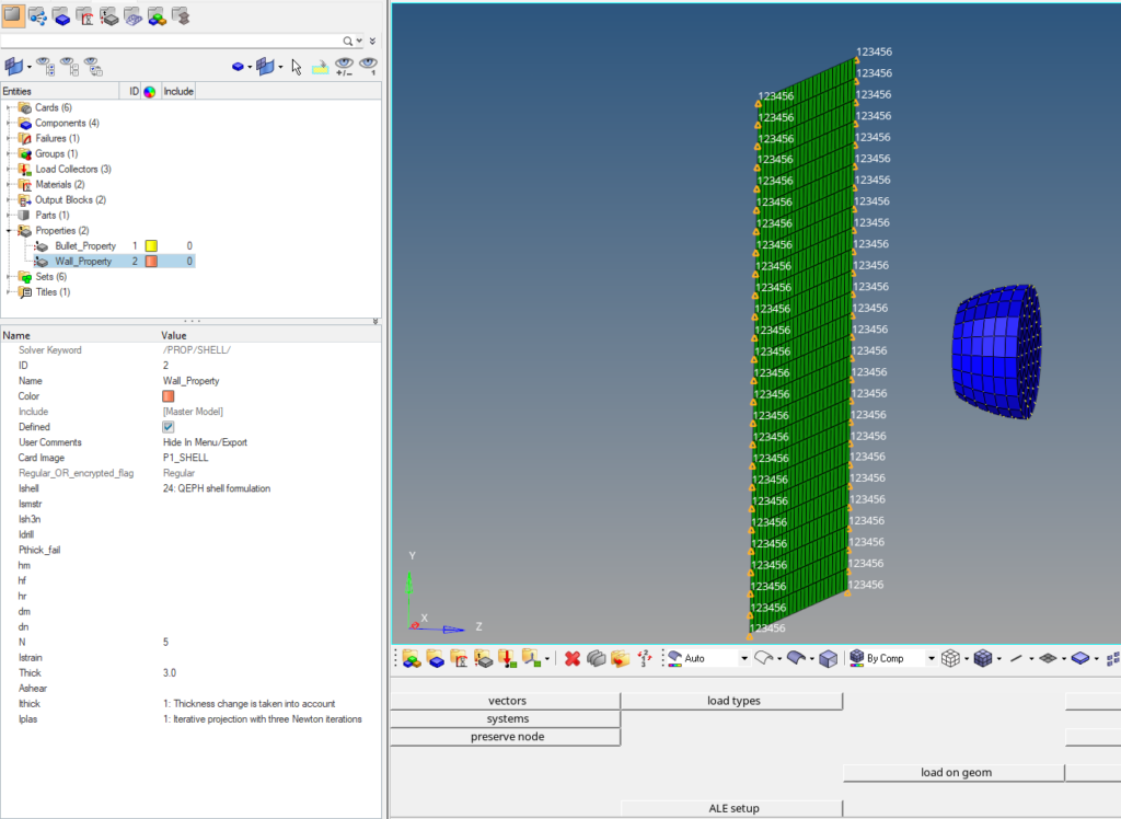
Next, we will create a PSHELL property by right-clicking on the white area on the browser area and selecting Create -> Property, we will name this property as Wall_Property, then select the card image as P1_SHELL, and put Ishell as “24 QEPH shell formulation”, N as 5, Thick as 3, Ithick as “1 Thickness change is taken into account”, Iplas as “1 Iterative projection with three Newton Iterations”, and assign this property to the bullet component. Refer to the image below for more clarity.
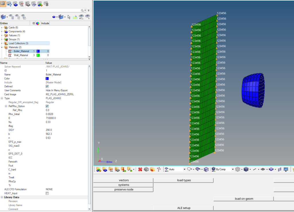
Then create a material by right-clicking on the white browser area and going to Create -> Material, we will name this material Bullet_Material, set the card image to M2_PLAS_JOHNS_ZERIL and the values for Rho_initial, E, Nu, SIGY, EPS_p_max, SIG_max() as shown in the image below.
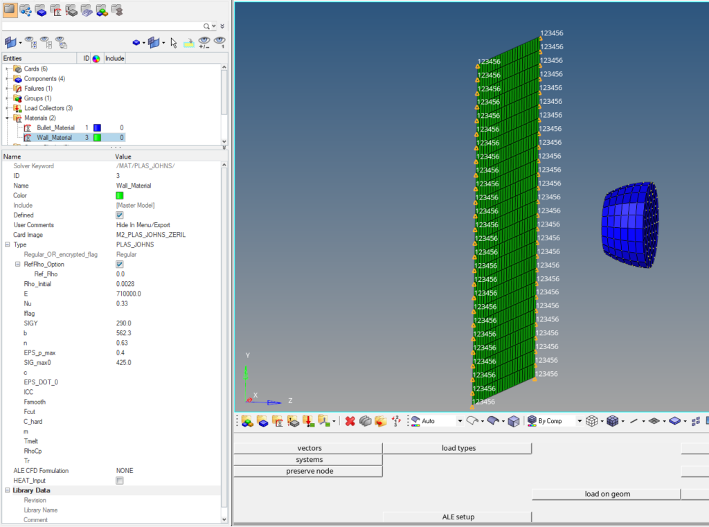
Then create a material by right-clicking on the white browser area and going to Create -> Material, we will name this material Wall_Material, set the card image to M2_PLAS_JOHNS_ZERIL and the values for Ref_Rho, Rho_initial, E, Nu, SIGY, b, n, EPS_p_max, SIG_max() as shown in the image below.
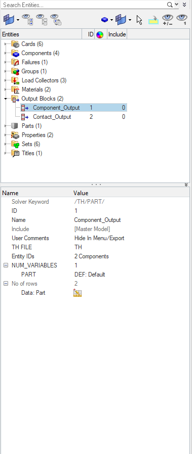
Next, we need to define the output blocks. We can do this by again right-clicking on the white-browser area and going to Create -> Output Blocks, we will name this output block Component_Output. Select the bullet and wall component under the Entity IDs field and NUM_Variables as 1. Refer to the below image.
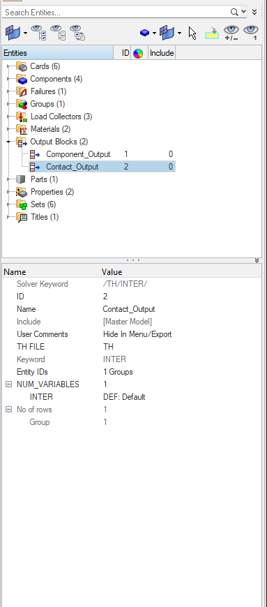
Next, we will create an output block for the contact. We can do this by again right-clicking on the white-browser area and going to Create -> Output Blocks, we will name this output block Contact_Output. Select the contact group under the Entity IDs field and NUM_Variables as 1. Refer to the below image.
Performing Analysis
First, we will select the output cards required for the analysis. We can do this by going to Analysis -> Control Cards. We will select the following cards and then assign the respective values in the respective fields.
- ENG_ANIM_DT – In Tfreq assign a value of 5e-05
- ENG_ANIM_ELEM – Select the EPSP, Energy, VONM, and HOURG fields.
- ENG_MON – Toggle the MON_ON_OFF to ON condition.
- ENG_RUN – In Tstop assign a value of 0.005.
- ENG_TFILE – In the type field use 0 built-in format of the current RADIOSS version, and in the Time_frequency field use 5e-05.
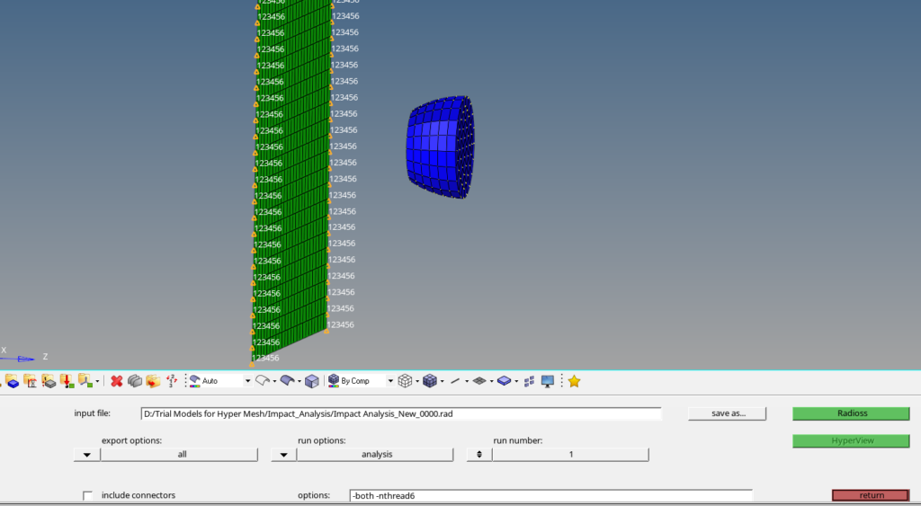
To perform the analysis go to Analysis -> Radioss, a window with the below image will appear. Kindly note that I am using Radioss here you can use any other non-linear solver of your choice. Click on Radioss to generate the Header and Engine file.
Now we need to run the Radioss solver. For this open the Radioss Solver and select the file ending with filename_0000, that is the header file. and then click on run to run the solver as shown in the image below.
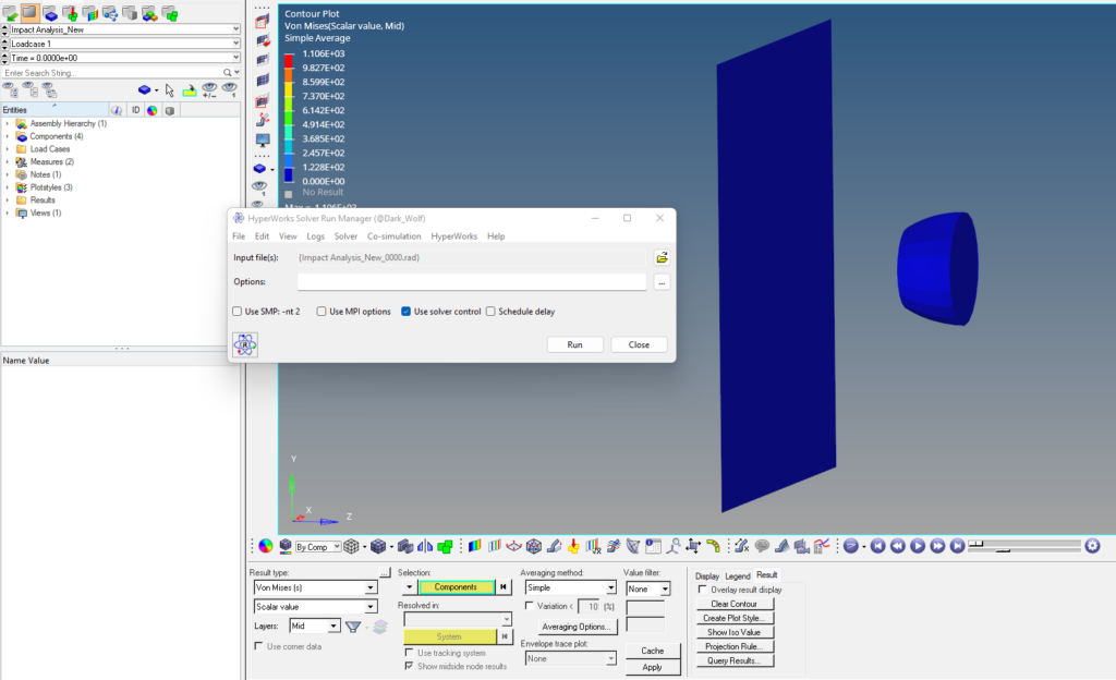
A pop-up window will open as shown in the image below:
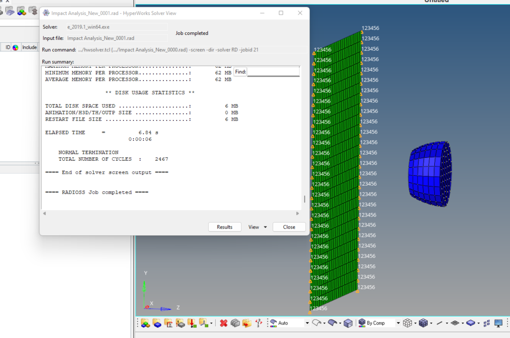
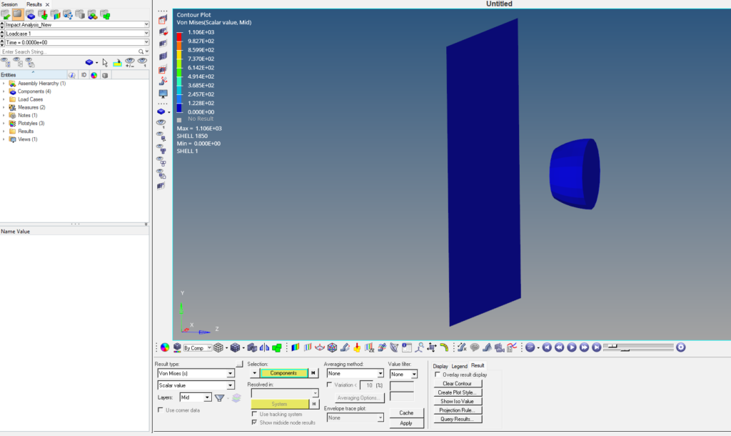
Output
Once the solver run is completed we can view the output values we can also go to View -> Output file. To visualize the results we can go to Results. This will open a Hyperview window. We can split the Hyperview window and visualize the results in both visual and graphical formats.
You can also refer to the video below for more clarity on the topic.
This is all for this post see you all in the next post. Don’t forget to follow my Facebook and Instagram Pages. Till then keep learning.