Till now we have seen how to mesh 2D and 3D elements and apply properties and materials to the components. In this post, we are going to look at the boundary conditions.
What are boundary conditions?
Boundary conditions are the conditions under which the body is simulated. Constraints or loads applied on the meshed components.
How do we decide these?
These inputs are given by the designer or the customer.
How do we apply them?
In Hypermesh under the Analysis field, there are options to apply constraints and loads.
Boundary Conditions -> Constraints:
To apply the constraints you can go to Analysis-> Constraints. Here you can constraint the different degrees of freedom for the nodes to be constrained. dof1 to dof3 are translational degrees of freedom, and dof4 to dof6 are rotational degrees of freedom. You can choose which degrees of freedom you want the node to have and what value to have in that. The card images available to be used in this are SPC, SPCD, etc.
You also have an option to apply MPC through Analysis-> Equations.
Now you would be wondering what are SPC, SPCD, and MPC.
SPC here stands for single-point constraint. It is used to constrain a node or a group of nodes for static or thermal analysis.
MPC here stands for Multipoint constraint. It is used to connect multiple independent nodes to a dependent node. You can define the degrees of freedom separately for the dependent and the independent node.
SPCD is used for defining velocity and acceleration for dynamic analysis in addition to the constraint options available in SPC.
Boundary Conditions -> Loads:
There are different options for Loads available in Hypermesh. Some of these are listed below:
- Forces: This is used to define a point load and can be applied to a node or a group of nodes. It applies a force on the selected nodes. The card images available for this type of load are FORCE, FORCE1, MBFRCC, and MBFRC. It can be applied by going to Analysis->Forces.
- Moments: This is also used to define a point load and can be applied to a node or a group of nodes. It applies moments on the selected nodes. The card images available for this type of load are MOMENT, MOMENT1, MBMNT, and MBMNTC. It can be applied by going to Analysis-> Moments.
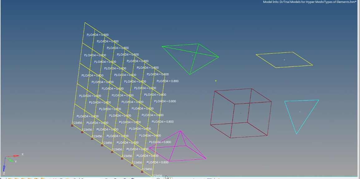
- Pressure: This is used to define surface load and can be applied to faces, elements, or edges. The card images available for this type of load are PLOAD, PLOAD1, PLOAD2, and PLOAD4. It can be applied by going to Analysis-> Pressure.
- Temperatures: This is used to apply concentrated temperature loads to nodes, surfaces, points, and lines.
- Flux: This is used to define flux loads at nodes. As the name suggests, flux means an amount of something passing through a unit area in a unit time, therefore this is particularly used for heat, mass, and fluid transfer analysis.
Now you must be thinking what is the use of these different card images. So let us understand the use of these different card images.
PLOAD is used to define load applied in static analysis on a 2D element. PLOAD1 is used to define load on CBAR and CBEAM elements which are 1D elements. PLOAD2 is used to define the load applied on a set of 2D elements. PLOAD4 is used to define load on 3D and 2D elements.
You can use a constant vector, curve, equations, linear interpolation, or nodally distributed options to define the magnitude of the Load.
Kindly note that the Force load affects only the dof1 to dof3 which are the translational degrees of freedom whereas the Moments affect the dof4 to dof6 which are the rotational degrees of freedom.
Loads and Constraints are defined in the model under the field Load collectors and applied through Load steps.
You can also refer to the below video to learn how to apply Loads and constraints.
This is all for this post, see you all in the next post. Don’t forget to follow my Facebook and Instagram pages for regular updates. Till then keep learning.