In the last post, we saw about system analysis. If you have not seen that post, you can check it out here. In this post, we will start with an analysis of an important part of the gun. Can you guess which part of the gun I am talking about?
If your guess was the barrel of a gun, then you are right? In this post, we are going to apply pressure load to the barrel of a Desert Eagle 0.5 magnum and observe its behaviour.
Disclaimer: This post is only for educational purposes, and the values used are not necessarily used for designing the firearm.
Performing Pressure Load Analysis
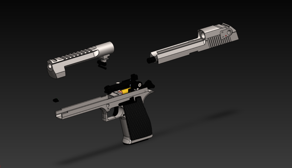
For this tutorial, we will use the barrel from a 0.44 Magnum Desert Eagle. The rationale for this analysis is that we are going to check how the barrel is going to behave under the instant burst of pressure generated while firing the bullet. The CAD model for the Desert Eagle is shown in the image below.
The Barrel of the Desert Eagle looks as follows:
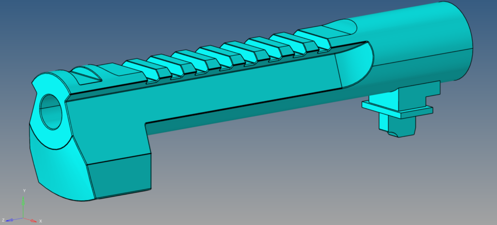
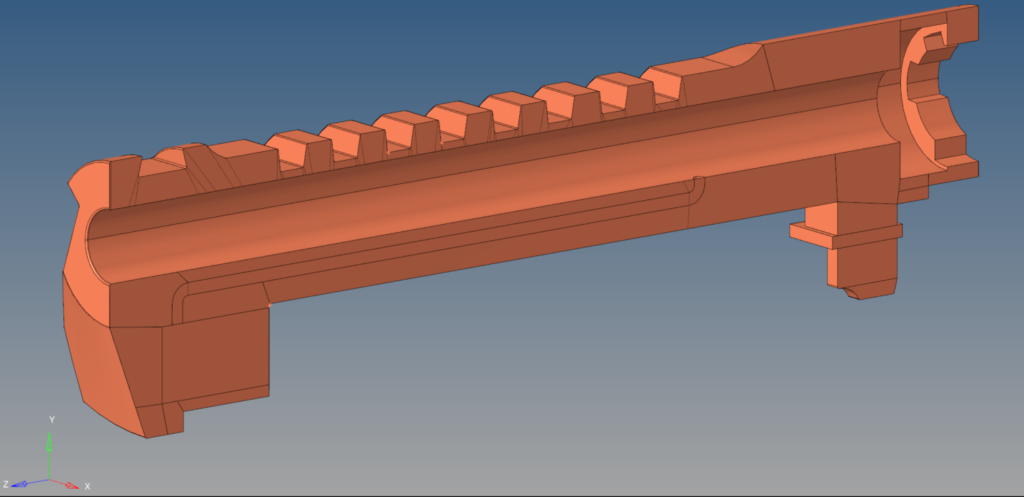
For this tutorial, I have taken a section of the barrel. We will be meshing this section of the barrel for analysis.
Meshed Model
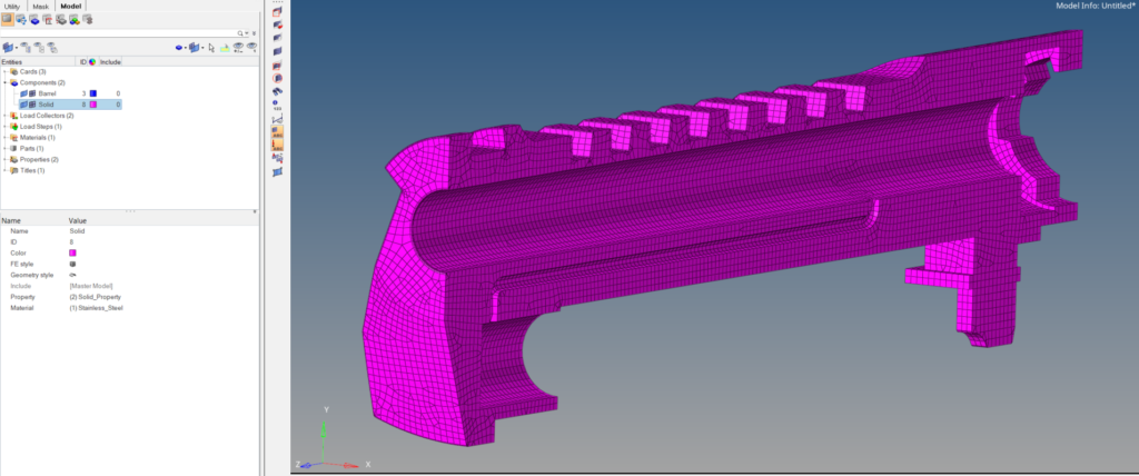
I have used the Barrel shown in the previous image and meshed it using 3D Tetra elements, as shown below:
Defining Property and Material
Now we need to define the material and properties for the meshed components. We will define the material first. For this, we will right-click the white browser area and then select Create -> Material. We will name this material Stainless Steel. Next, we will enter the material values as shown in the image below.
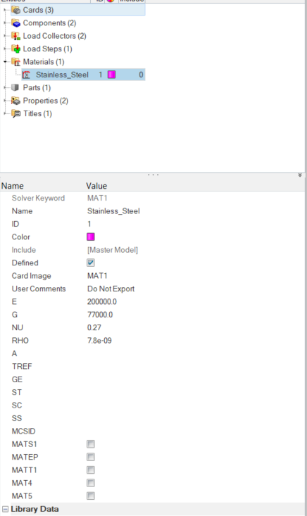
Kindly note that the values used for this tutorial are only for educational purposes and are not necessarily the real values of the material used while designing the firearm.
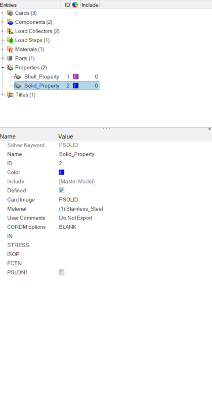
Next, we need to define the property for the meshed component. For this, we will right-click the white browser area and then select Create -> Property. We will name this property Solid_Property as shown in the image below.
Boundary Condition
To apply boundary conditions, we have to first create load collectors for the same. We can right-click on the white browser area and then go to Create -> Load Collector. We will name this load collector the Static_Load. Then, to create the pressure load, we can go to Analysis -> Pressures, and then select the elements on which the pressure load will be applied, i.e., the elements on the inner face of the barrel, as shown in the image below. We will keep the pressure value at 225 MPa. Refer to the image shown below.
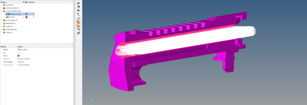
Kindly note that the values used for this tutorial are only for educational purposes and are not necessarily the real values used while designing the firearm.
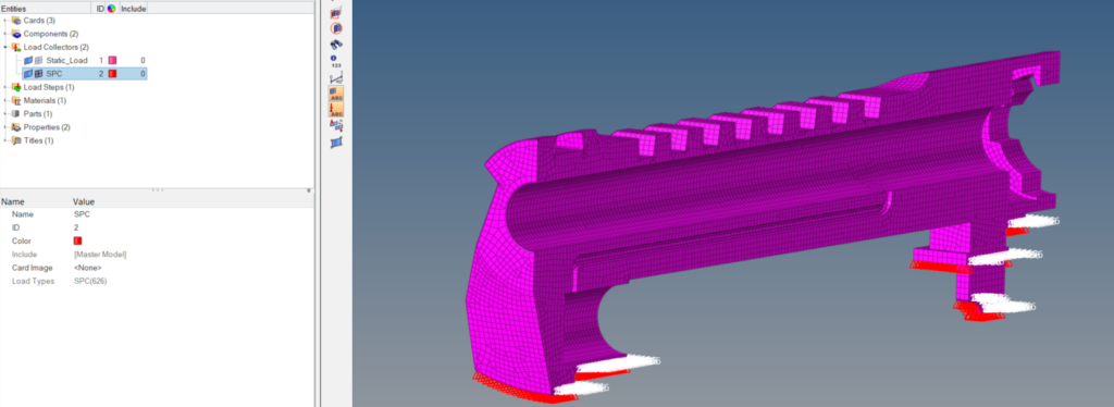
Next, we need to create a constraint for the barrel. For this, we can again right-click on the white browser area and then go to Create -> Load Collector. We will name this load collector the SPC. Then, to create the constraints, we can go to Analysis -> Constraints, and then select all the degrees of freedom and the elements on the face which will get connected to the frame of the gun. Refer to the image shown below.
Analysis Setup
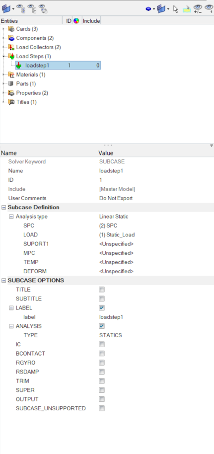
Next, we will create a Load Step by right-clicking on the white browser area and then going to Create -> Load step. We will name this load step as loadstep1. We will change the analysis type from generic to Linear Static, and then we will reference the Static_Load load collector under the Load field and the SPC load collector under the SPC field.
After this, we need to define the control cards for the analysis to take place. We can do this by going to Analysis -> Control Cards -> Solution. We have to select SOL 101 for this case.
Then we need to select the parameter for the solver. We can do this by going to Analysis -> Control Cards -> PARAM. We will select AUTOSPC as Yes, WTMASS as 0.001 and POST as 1.
Then we need to select Output requests. For this, we can go to Analysis -> Control Cards ->Global Output Requests. We will select Displacement, Stress and Strain here.
Performing Analysis
To perform the analysis, we need to export the BDF file. We can do this by going to File -> Export and selecting the export format and location, and then clicking on Export. After this, open the Nastran solver and select the file. The result of the analysis run will be similar to the images shown below.
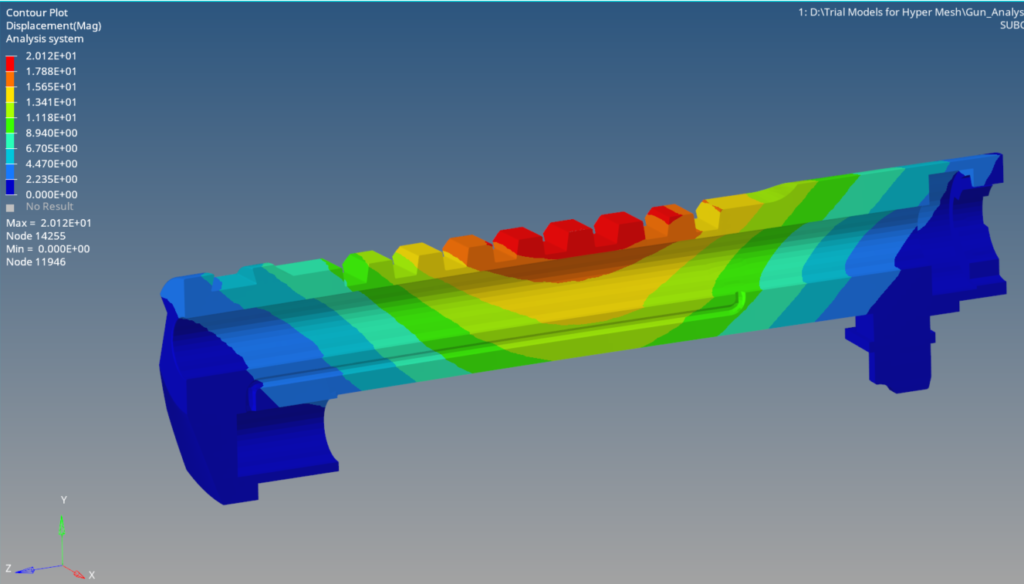
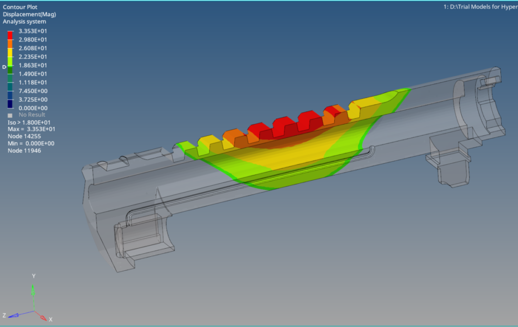
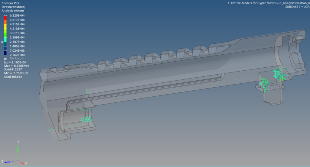
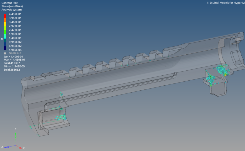
Kindly note that the results for this tutorial are only for educational purposes and are not necessarily the real results generated while designing the firearm.
Refer to the video below for better clarity.
This is all for this post. Don’t forget to follow my Facebook and Instagram pages for regular updates. See you all in the next post. Till then, keep learning.