In the previous posts, we have seen different types of analyses. If you have not seen them, you can see them here. This post is going to be a bit different. We are going to explore the Hyperview Interface.
So, to start with, first of all, let’s understand what Hyperview is.
Hyperview is a post-processor offered by Altair under the HyperWorks package. It is used to view and analyze the results produced by the solver for the Finite Element Model.
Interface of Hyperview
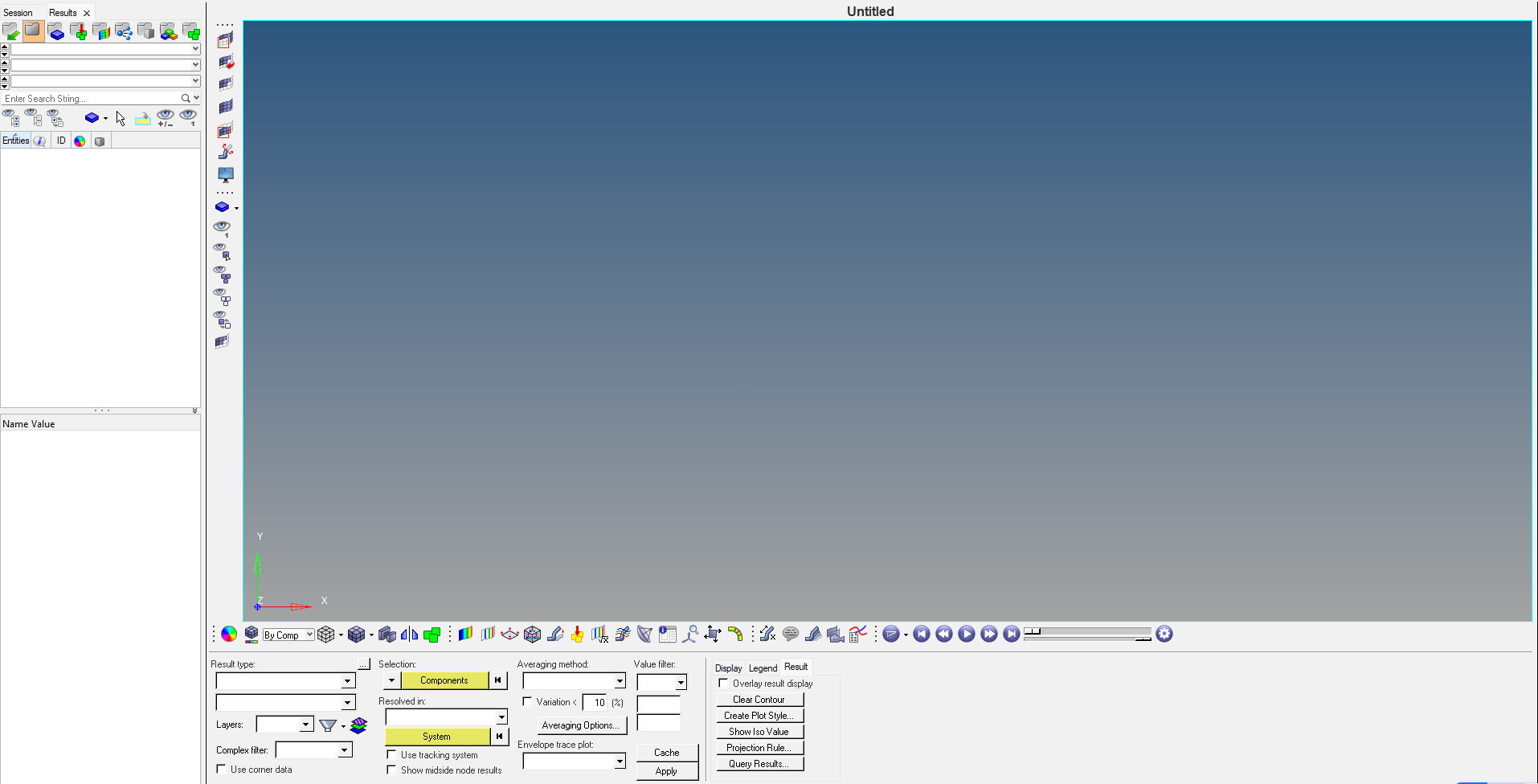
The Interface of Hyperview looks as shown below:
The white browser area on the left side is the same as Hypermesh. Here you can view your components, contacts, Load collectors, etc. The main focus and the part where Hyperview differs from Hypermesh are the panels that are available in it.
The different types of panels available in Hyperview are as follows:
1. Contour Panel
The Contour Panel in HyperView is a powerful visualization tool used to display and analyze results from finite element analysis (FEA). It helps us interpret simulation data by mapping values—like stress, strain, displacement, temperature, etc. onto the geometry of the model using color gradients.
Key Uses of the Contour Panel in HyperView
- Visualize Simulation Results – Display results as color-coded plots on the model surface. Supports both nodal and elemental results, including corner results.
- Select Result Types – Choose from various result types like: Displacement (vector), Stress/Strain (tensor), Temperature, Energy, Porosity (scalar), Customize which component to display (e.g., X, Y, Z, von Mises, MaxShear).
- Manage Display Options – Control how contours appear: Continuous vs. Discontinuous, Smooth shading vs. flat, Iso-value display, Section cuts, and overlays.
- Layer-Specific Visualization – If your model has layered elements (like composites), you can display contours for specific layers.
- Query and Analyze – Click on parts of the model to get exact values. Use legends to interpret the range and distribution of results.
For example, in the below example of static analysis of beam . Using the Contour Panel, you can:
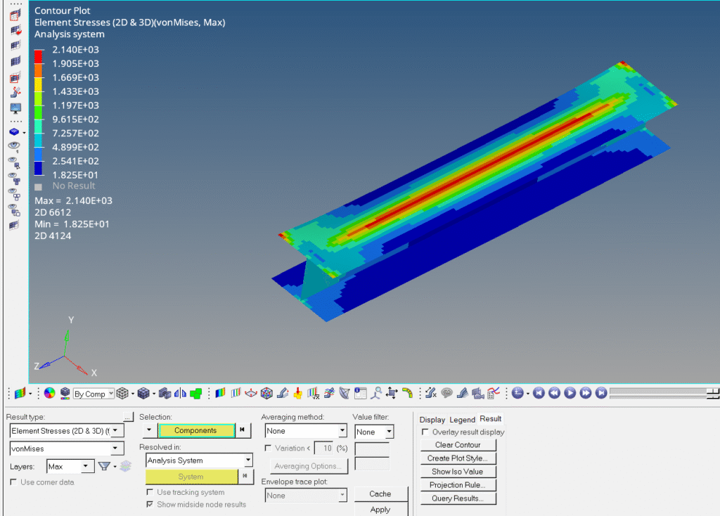
- Select Stress → von Mises, Signed von Mises.
- View high-stress zones in red and low-stress zones in blue.
- Identify potential failure points or areas needing design changes.
If you’re working with ANSYS .rst or .cdb files, HyperView supports direct visualization of those results too.
2. Iso
The Iso Panel in HyperView is a specialized tool used to display iso surfaces or iso lines—regions in your model where a particular result value (like stress, pressure, or temperature) remains constant. It’s especially useful for visualizing critical thresholds and identifying hotspots in simulation data.
Key uses of Iso Panel
1. Create Iso Surfaces or Iso Lines – For solid elements, it generates iso surfaces (3D). For shell elements, it creates iso lines (2D). These represent areas where the result value equals a specific threshold.
2. Focus on Specific Result Values – You can select a result type (e.g., pressure, stress) and set a target value. The model will highlight only those regions that match or exceed that value. Useful for pinpointing failure zones or design limits.
3. Combine with Contour Plots – You can overlay contour plots on top of iso surfaces to get dual-layer insight. For example, show density iso surfaces and stress contours simultaneously to analyze optimized designs.
4. Interactive Exploration – Use the slider bar to dynamically adjust the iso value and watch how the highlighted region changes. This helps in understanding how sensitive your model is to certain thresholds.
5. Transparent Geometry View – Combine iso surfaces with transparent boundary geometry (shortcut key "T") for an X-ray-like view of internal stress or pressure zones.
For example, in the image below, you can see the beam from the static analysis.
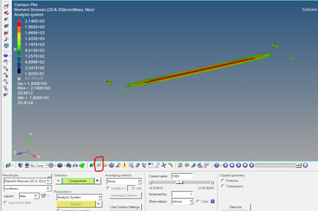
- You set the iso value to 1000 MPa.
- The Iso Panel highlights all regions where pressure equals 1000 MPa.
3. Vector
The Vector Panel in HyperView is used to create and customize vector plots—graphical representations of vector-based results like displacement, velocity, or acceleration—mapped onto your model. These plots help you understand the direction, magnitude, and distribution of forces or movements across the structure.
Key Uses of the Vector Panel
1. Visualize Vector Fields – Display vectors at nodes to show how the model moves or reacts. Common result types:
- Displacement vectors (how far and in which direction nodes move)
- Velocity vectors (speed and direction of movement)
- Acceleration vectors (rate of change of velocity)
2. Customize Display Settings – Choose which components to show: X, Y, Z, or resultant (X+Y+Z). Adjust vector size scaling, color mapping, and system of resolution (global vs. local). Color vectors by direction or magnitude to highlight patterns.
3. Interactive Analysis – Select specific nodes or regions to focus on. Use window selection or pick nodes manually. Overlay vector plots with contour plots for deeper insight.
4. Compare Systems – Resolve vectors in different coordinate systems (e.g., global, local, analysis). Useful when analyzing complex assemblies with multiple reference frames.
Refer to the image below:
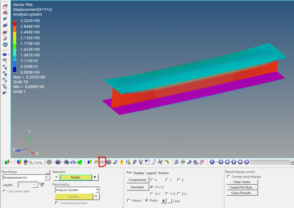
- Use the Vector Panel to plot displacement vectors.
- See how different parts of the vehicle deform and in which direction.
- Color by magnitude to identify areas of maximum movement.
4. Tensor
The Tensor Panel in HyperView is designed to visualize tensor data—such as stress and strain tensors—in a way that reveals both magnitude and directionality across your model. This is especially useful when analyzing complex mechanical behaviors in simulations from solvers like ANSYS, Nastran, or OptiStruct.
What Is Tensor Data?
A tensor is a mathematical object that describes multi-directional quantities. In FEA, stress and strain are typically represented as second-order tensors, meaning they have components in multiple directions (e.g., XX, YY, ZZ, XY, etc.).
Key Uses of the Tensor Panel
1. Visualize Principal Directions – Displays principal stress or strain directions as arrows or glyphs. Helps identify how forces are distributed and oriented within the material.
2. Analyze Magnitude and Orientation – Shows both the magnitude of tensor components and their direction. Useful for spotting areas of high shear, tension, or compression.
3. Support for Elemental Results – Works with elemental values from various solvers. Ideal for post-processing results from structural, thermal, or fluid simulations.
4. Enhanced Interpretation – Complements contour and vector plots by adding directional context. Especially valuable in anisotropic materials or composite structures.
Refer to the image below:
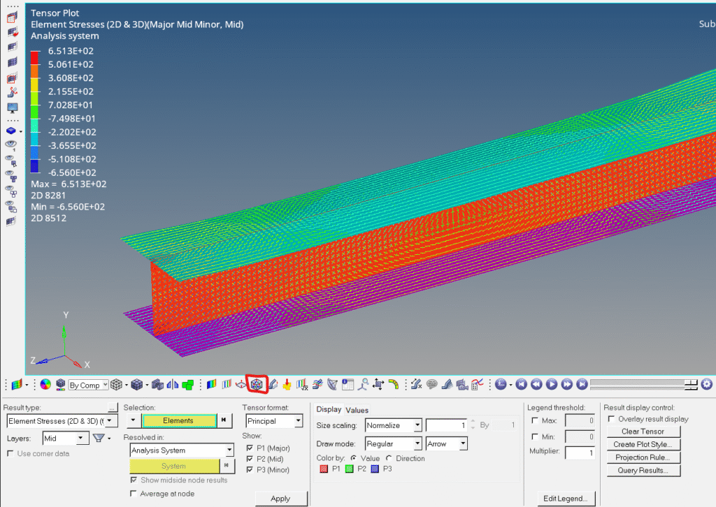
- Use the Tensor Panel to view principal stress directions.
- See how fibers align with stress paths.
- Identify potential failure zones due to misaligned stress vectors.
5. Deformed
The Deformed Panel in HyperView is your go-to tool for visualizing how a structure changes shape under load, impact, or other physical conditions. It lets you animate and inspect the deformed geometry of your model based on simulation results—essential for understanding how your design behaves in the real world.
Key Uses of the Deformed Panel
1. Display Deformed Shapes – Shows how the model physically deforms under applied loads. You can view the original shape, the deformed shape, or both overlaid to compare.
2. Animate Structural Motion – Create animations of the deformation across time steps or modes. Useful for transient, modal, or interpolation-based simulations.
3. Control Scale Factor – Adjust the deformation scale to exaggerate or normalize the visual effect. Helps highlight subtle movements or avoid misleading exaggerations.
4. Choose Result Type – Select from available nodal vector results like displacement, velocity, or acceleration. Tailor the deformation display to the specific analysis you’re performing.
5. Export Deformed Geometry – Export the deformed shape for use in other tools or documentation. Supports formats like Abaqus, OptiStruct, Nastran, RADIOSS, and STL.
Refer to the image below:
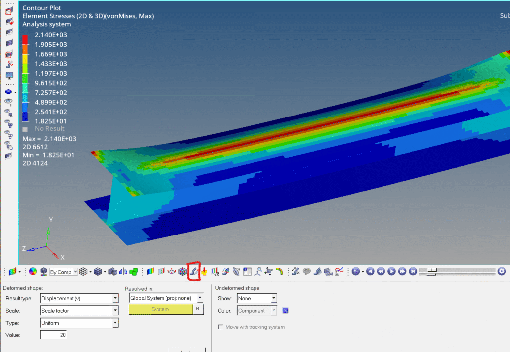
- Use the Deformed Panel to animate how the bridge bends.
- Overlay the original and deformed shapes to see where the most movement occurs.
- Export the deformed shape for further CAD or mesh refinement.
6. Derived Load Steps
The Derived Load Step Panel in HyperView is a powerful feature that lets you create customized combinations of simulation results—especially useful when you’re working with multiple load cases or time steps and want to extract meaningful insights across them.
What You Can Do with the Derived Load Step Panel
1. Create Custom Load Cases – Combine results from multiple load steps (e.g., different time frames, load conditions) into a single derived case. Useful for evaluating worst-case scenarios, envelopes, or averaged responses.
2. Envelope Calculations – Generate envelope plots that show the maximum or minimum value across selected steps. Ideal for identifying peak stress, displacement, or temperature across a range of conditions.
3. User-Defined Expressions – Define custom mathematical expressions using existing result types. For example, you could compute a derived result like:von Mises stress × safety factor + thermal expansion
4. Streamlined Post-Processing – Instead of manually switching between load steps, you can automate comparisons and visualize results in one go. Saves time and reduces errors in interpreting complex simulations.
5. Animation and Tracking – Animate derived results over time or across load cases. Track specific entities (nodes, elements) to see how they behave under combined conditions.
Imagine you’re analyzing an aircraft wing under multiple flight conditions:
- Use the Derived Load Step Panel to create an envelope of maximum stress across all load cases.
- Visualize this in a single contour plot to identify critical regions.
- Export the derived case for reporting or further analysis.
7. Derived Results
The Derived Panel in HyperView is a powerful tool that allows you to create custom result types by applying mathematical expressions to existing simulation data. It’s especially useful when you want to go beyond standard outputs like stress or displacement and generate user-defined results tailored to your analysis needs.
Key Uses of the Derived Panel
1. Create Custom Results Using Expressions – Use the Expression Builder to define new results based on existing ones. For example:Derived_Stress = von_Mises_Stress × Safety_Factor + Thermal_Expansion
2. Combine Multiple Load Cases – Generate results that span across multiple load steps or subcases. Useful for comparing or combining results from different conditions (e.g., subtracting stress at Loadcase 1 from Loadcase 2).
3. Envelope and Extremum Calculations – Create maximum, minimum, or average results across selected load steps. Ideal for identifying worst-case scenarios or performance envelopes.
4. Advanced Post-Processing – Apply logical, arithmetic, and statistical operations to simulation data. Supports Templex-style syntax and XML-based result math processing.
5. Make Results Available Across Panels – Once created, derived results can be used in:
- Contour plots
- Vector plots
- Tensor plots
- Animations
Imagine you’re analyzing a composite panel under thermal and mechanical loads:
- Use the Derived Panel to compute a combined failure index based on stress and temperature.
- Visualize this result in the Contour Panel to identify critical zones.
- Animate the derived result over time to track performance degradation.
8. Streamlines
The Streamline Panel in HyperView is a specialized tool used primarily for CFD (Computational Fluid Dynamics) post-processing. It allows you to visualize flow patterns by generating streamlines—paths that represent the trajectory of particles moving through a vector field like velocity or pressure.
Key Uses of the Streamline Panel
1. Visualize Flow Direction and Behavior – Streamlines show how fluid (air, water, etc.) moves through and around your model. Ideal for analyzing aerodynamics, thermal flows, or internal fluid movement.
2. Generate Streamlines from Vector Fields – Use nodal or elemental vector data (typically velocity fields) to create streamlines. Supported by solvers like AcuSolve, Fluent, RADIOSS, and others via EnSight files.
3. Animate Particle Movement – You can animate particles traveling along streamlines to simulate real-time flow. Useful for visualizing dust, smoke, or fluid particles in motion.
4. Customize Rakes and Streamline Sources – Define rakes (line, area, or plane sources) where streamlines originate. Control the number, spacing, and orientation of streamlines for precise analysis.
5. Apply Contours to Streamlines – Overlay scalar results (like pressure or temperature) as contours on streamlines. Enhances insight into how flow interacts with other physical phenomena.
Imagine you’re analyzing airflow over a car body:
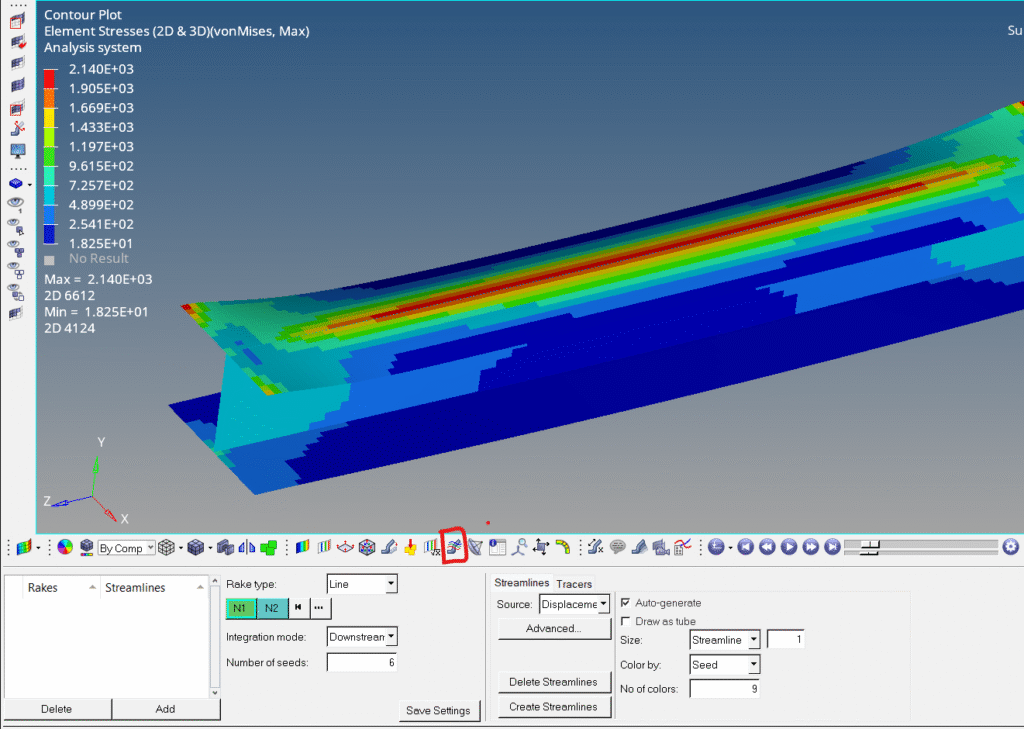
- Use the Streamline Panel to generate flow paths from the front grille.
- Animate particles to see how air moves over the hood and roof.
- Apply pressure contours to streamlines to identify drag zones and optimize design.
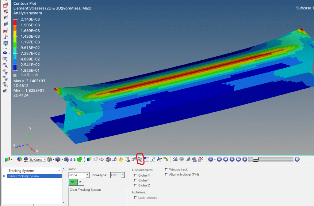
9. Tracking Systems
The Tracking System Panel in HyperView is a dynamic visualization tool that allows you to lock the camera view onto a moving entity during animation. This is especially useful when analyzing motion, deformation, or interaction between parts in simulations like crash tests, drop analyses, or multi-body dynamics.
Key Uses of the Tracking System Panel
1. Track Entities During Animation – Keeps the selected entity (node, element, or component) centered and stable in the view as it moves. Makes it easier to observe relative motion, rotations, or displacements without manually adjusting the camera.
2. Model-Based vs. Window-Based Tracking
- Model-Based: Tracking system is tied to a specific model.
- Window-Based: Allows tracking across multiple models in the same window—ideal for overlay comparisons.
3. Compare Deformations Across Models – When overlaying two models (e.g., baseline vs. modified design), you can define separate tracking systems for each. Helps in shape comparison and motion analysis between versions.
4. Coordinate System Alignment – You can align the tracking system with global or local coordinate systems. Useful for transforming outputs back to global directions or analyzing motion in a specific frame of reference.
5. Manage Multiple Tracking Systems – Create, rename, activate/deactivate, and delete tracking systems. Easily switch between tracking setups depending on what part of the model you want to follow.
Imagine you’re analyzing a vehicle crash simulation:
- Use the Tracking System Panel to follow the front bumper as it deforms.
- The camera stays locked on the bumper, making it easier to observe how it crumples and interacts with other parts.
- Overlay a second model with a different material and track the same region for comparison.
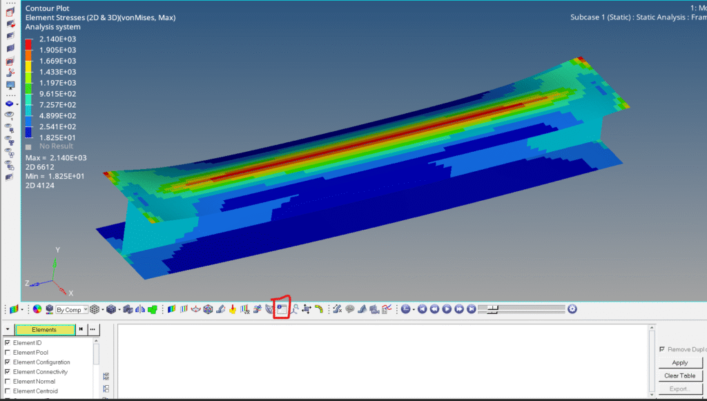
10. Query
The Query Panel in HyperView is a versatile tool designed to help you inspect, filter, and export detailed information about entities in your simulation model—such as nodes, elements, components, and systems. It’s especially useful when you need to dig into the numerical data behind your visual results.
Key Uses of the Query Panel
1. View Entity Properties – Inspect attributes like:
- Node coordinates
- Element connectivity
- Component IDs and names
- System definitions
- Helps verify model setup and troubleshoot inconsistencies.
2. Filter and Select Entities – Use advanced filters to create selection sets based on specific criteria. For example, select all elements with stress above a certain threshold or nodes within a defined region.
3. Export Data Tables – Export queried data to CSV or Excel for reporting or further analysis. Ideal for documenting results or integrating with external tools.
4. Create Groups or Sets – Turn queried entities into named sets for use in other panels (e.g., contour, vector, tensor). Useful for isolating critical regions or tracking specific components.
5. Context Menu and Table Tools – Right-click to access context-sensitive options like Sorting, Copying, Saving, Importing external data for comparison
Imagine you’re analyzing a crash simulation:
- Use the Query Panel to extract all nodes in the front bumper region.
- Filter for nodes with displacement > 50 mm.
- Export the data to Excel for a report on deformation zones.
Refer to the video below for more clarity.
We will continue the rest in the next post.
This is all for this post. I hope you learned something from this post. Don’t forget to follow my Facebook and Instagram Pages for regular updates. See you all in the next post. Till then, keep learning.