In one of the previous posts, we have performed static analyses. You can check those posts out here if you have not seen them. In this post, we will conduct a Crash Analysis using Hypermesh and Radioss.
We will start with understanding what is Crash Analysis, and what leads to these loads and then finally prepare a model and perform the analysis.
What is Crash Analysis?
Crash Analysis as the word states is used to study the effect on the body when it collides with a rigid body or surface. The thing we will observe here is how energy is dissipated and how the stress is transferred. If you would have studied elementary physics you would know that there are two types of collisions, namely elastic and inelastic collision, and there is an exchange or transfer of energy during collision.
This analysis is more relevant in the automotive industry. Making a full-size vehicle and then performing a destructive test on it again is a costly affair. Therefore Crash analysis is used there to save time and cost.
Performing Crash Analysis
For this tutorial, we will use a 9 mm bullet traveling at a speed of 50 m/s and observe the effect on the bullet when it collides with a rigid wall.
Meshed Model
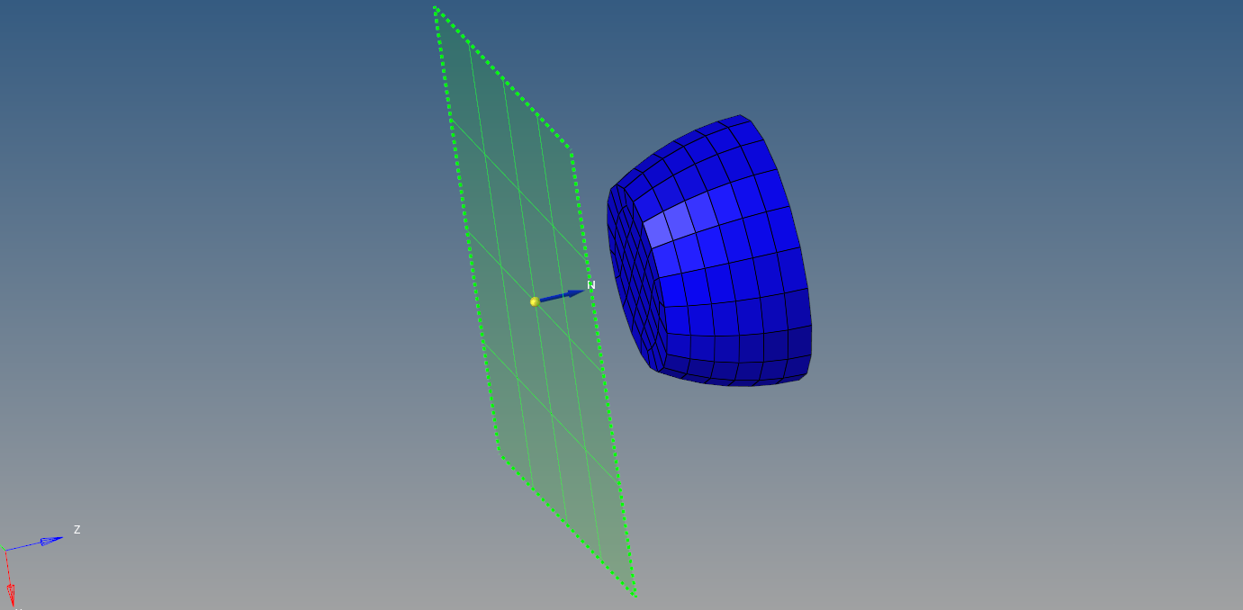
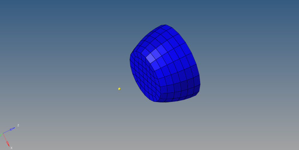
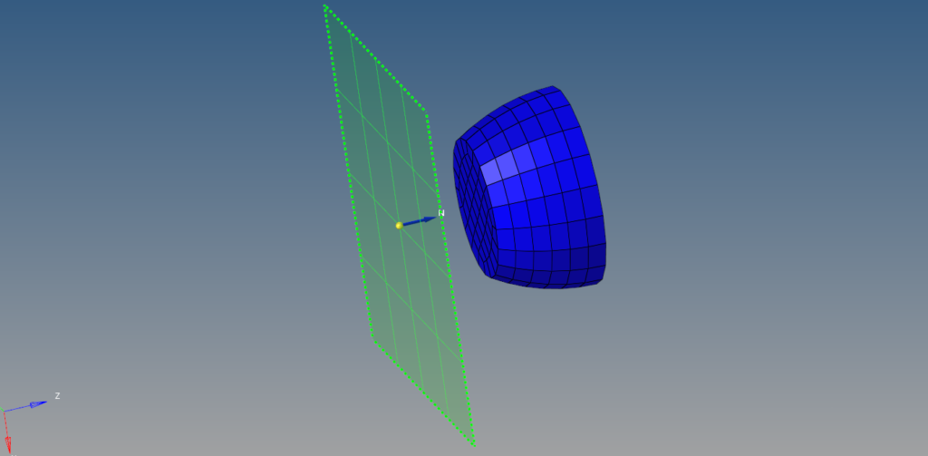
In this tutorial, we will be using a 9 mm bullet meshed with 2D elements of mixed type, the bullet is traveling at a speed of 50 m/s as shown in the image below:
Boundary Conditions
Post meshing the bullet we need to give the boundary conditions.
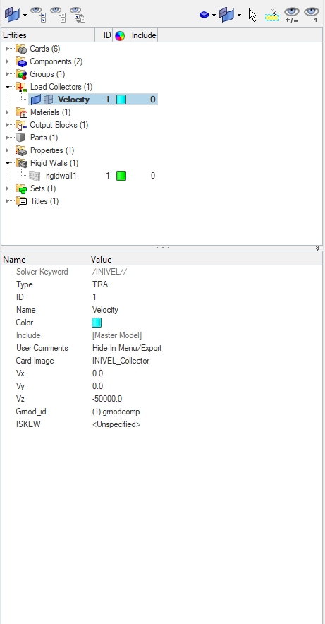
Here we will give the bullet an initial velocity of 50 m/s. For this, we can go to Tools -> BCs Manager and create the initial velocity Load Collector, select the bullet component to assign velocity to it. Here I have used the velocity as -50000 in the z field as the bullet is pointing towards negative Z-direction and the unit of velocity is mm/s in Hypermesh as shown in the below image.
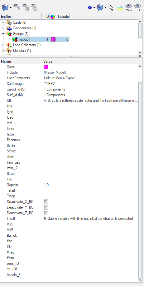
Next, we will need to define the contacts for the bullet. For this, we can right-click on the white browser area and then go to Create -> Contact. Here we will select the card image of contact as TYPE 7, the bullet component as the slave as well as the master entity, and Istf (stiffness definition) as 4. Stfac is a stiffness scale factor and the interface stiffness is computed from both master and slave characteristics, Gapmin as 1, and Inacti as 6 Gap is variable with time but initial penetration is computed.
Analysis Setup
We have to now apply material, property, and create load step.
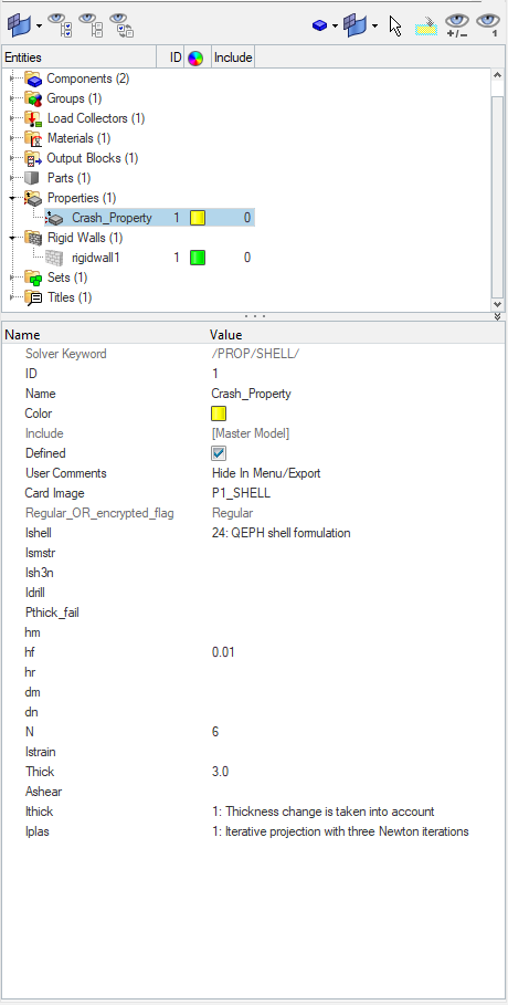
Create a PSHELL property by right-clicking on the white area on the browser area and selecting Create -> Property, then select the card image as P1_SHELL, and put Ishell as 24 QEPH shell formulation, hf as 0.01, N as 6, Thick as 3, Ithick as 1 Thickness change is taken into account, Iplas as 1 Iterative projection with three Newton Iterations, and assign this property to the bullet component. Refer to the image below for more clarity.
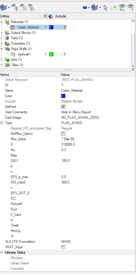
Then create a material by right-clicking on the white browser area and going to Create -> Material, set the card image to M2_PLAS_JOHNS_ZERIL and the values for Rho_initial, E, Nu, SIGY, EPS_p_max, SIG_max() as shown in the image below.
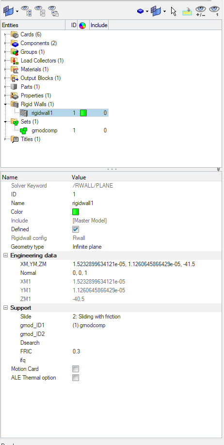
Next, we have to create a Rigid wall. For this, we will again right-click on the white-browser area and go to Create -> Rigid Wall. For assigning the coordinates for the rigid wall we first need to create a temporary node at a distance of 5mm from the bullet and then assign the normal vector as z direction as shown in the image below. Select the velocity set under gmod_ID1, Slide as 2 Sliding with friction and FRIC as 0.3. Refer to the below image.
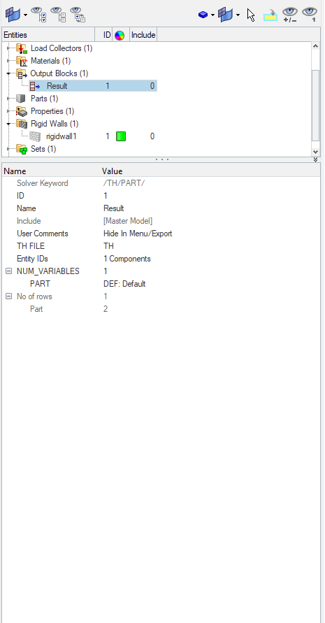
Next, we need to define the output block. We can do this by again right-clicking on the white-browser area and going to Create -> Output Blocks. Select the bullet component under the Entity IDs field and NUM_Variables as 1. Refer to the below image.
Performing Analysis
First, we will select the output cards required for the analysis. We can do this by going to Analysis -> Control Cards. We will select the following cards and then assign the respective values in the respective fields.
- ENG_ANIM_DT – In Tfreq assign a value of 8e-05
- ENG_ANIM_ELEM – Select the EPSP, Energy, VONM, and HOURG fields.
- ENG_MON – Toggle the MON_ON_OFF to ON condition.
- ENG_RUN – In Tstop assign a value of 0.008.
- ENG_TFILE – In the type field use 0 built-in format of the current RADIOSS version, and in the Time_frequency field use 4e-5.
To perform the analysis go to Analysis -> Radioss, a window with the below image will appear. Kindly note that I am using Radioss here you can use any other non-linear solver of your choice. Click on Radioss to generate the Header and Engine file.
Now we need to run the Radioss solver. For this open the Radioss Solver and select the file ending with filename_0000, that is the header file. and then click on run to run the solver as shown in the image below.
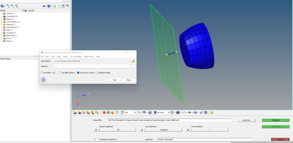
A pop-up window will open as shown in the image below:
Output
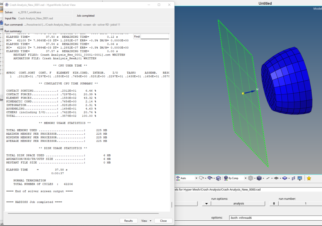
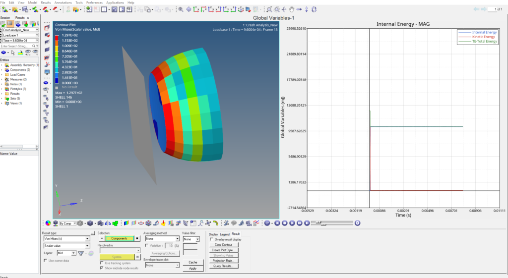
Once the solver run is completed we can view the output values we can also go to View -> Output file. To visualize the results we can go to Results. This will open a Hyperview window. We can split the Hyperview window and visualize the results in both visual and graphical formats.
You can refer to the video below for more clarity on the topic.
This is all for this post see you all in the next post. Don’t forget to follow my Facebook and Instagram Pages. Till then keep learning.